|
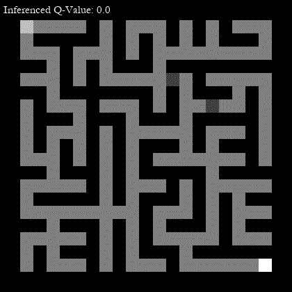
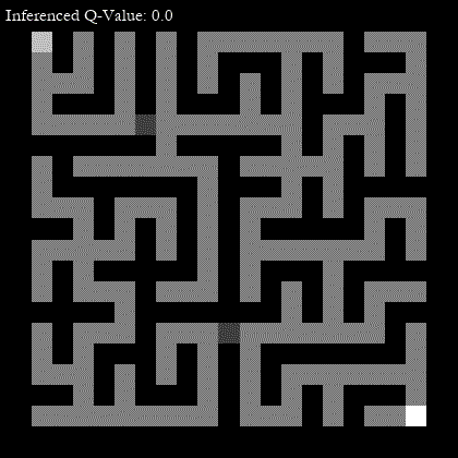
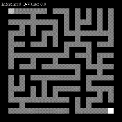
Deep Reinforcement Learning (Deep Q-Network: DQN) to solve Maze. |
Multi-agent Deep Reinforcement Learning to solve the pursuit-evasion game. |
|
Deep Reinforcement Learning (Deep Q-Network: DQN) to solve Maze. |
Multi-agent Deep Reinforcement Learning to solve the pursuit-evasion game. |
 that is probability that agent searches greedy. Greedy searching is *deterministic* in the sense that policy of agent follows the selection that maximizes the Q-Value.
Boltzmann Q-Learning algorithm is based on Boltzmann action selection mechanism, where the probability
that is probability that agent searches greedy. Greedy searching is *deterministic* in the sense that policy of agent follows the selection that maximizes the Q-Value.
Boltzmann Q-Learning algorithm is based on Boltzmann action selection mechanism, where the probability
 of selecting the action
  is given by
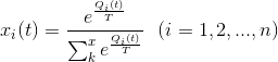
 controls exploration/exploitation tradeoff. For
  the agent always acts greedily and chooses the strategy corresponding to the maximum Q–value, so as to be pure *deterministic* exploitation, whereas for
  the agent’s strategy is completely random, so as to be pure *stochastic* exploration.
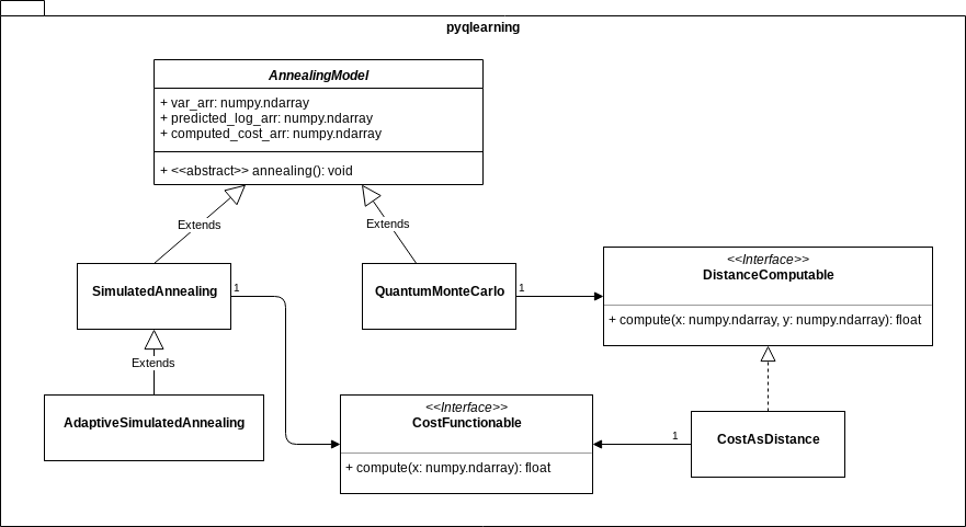
### Commonality/variability of Q-learning models
Considering many variable parts and functional extensions in the Q-learning paradigm from perspective of *commonality/variability analysis* in order to practice object-oriented design, this library provides abstract class that defines the skeleton of a Q-Learning algorithm in an operation, deferring some steps in concrete variant algorithms such as Epsilon Greedy Q-Leanring and Boltzmann Q-Learning to client subclasses. The abstract class in this library lets subclasses redefine certain steps of a Q-Learning algorithm without changing the algorithm's structure.
the agent’s strategy is completely random, so as to be pure *stochastic* exploration.
### Commonality/variability of Q-learning models
Considering many variable parts and functional extensions in the Q-learning paradigm from perspective of *commonality/variability analysis* in order to practice object-oriented design, this library provides abstract class that defines the skeleton of a Q-Learning algorithm in an operation, deferring some steps in concrete variant algorithms such as Epsilon Greedy Q-Leanring and Boltzmann Q-Learning to client subclasses. The abstract class in this library lets subclasses redefine certain steps of a Q-Learning algorithm without changing the algorithm's structure.
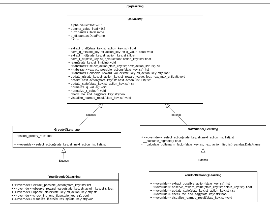 Typical concepts such as `State`, `Action`, `Reward`, and `Q-Value` in Q-learning models should be refered as viewpoints for distinguishing between *commonality* and *variability*. Among the functions related to these concepts, the class `QLearning` is responsible for more *common* attributes and behaviors. On the other hand, in relation to *your* concrete problem settings, more *variable* elements have to be implemented by subclasses such as `YourGreedyQLearning` or `YourBoltzmannQLearning`.
For more detailed specification of this template method, refer to API documentation: [pyqlearning.q_learning module](https://code.accel-brain.com/Reinforcement-Learning/pyqlearning.html#module-pyqlearning.q_learning). If you want to know the samples of implemented code, see [demo/](https://github.com/chimera0/accel-brain-code/tree/master/Reinforcement-Learning/demo).
### Structural extension: Deep Reinforcement Learning
The Reinforcement learning theory presents several issues from a perspective of deep learning theory(Mnih, V., et al. 2013). Firstly, deep learning applications have required large amounts of hand-labelled training data. Reinforcement learning algorithms, on the other hand, must be able to learn from a scalar reward signal that is frequently sparse, noisy and delayed.
The difference between the two theories is not only the type of data but also the timing to be observed. The delay between taking actions and receiving rewards, which can be thousands of timesteps long, seems particularly daunting when compared to the direct association between inputs and targets found in supervised learning.
Another issue is that deep learning algorithms assume the data samples to be independent, while in reinforcement learning one typically encounters sequences of highly correlated states. Furthermore, in Reinforcement learning, the data distribution changes as the algorithm learns new behaviours, presenting aspects of *recursive learning*, which can be problematic for deep learning methods that assume a fixed underlying distribution.
#### Generalisation, or a function approximation
This library considers problem setteing in which an agent interacts with an environment
Typical concepts such as `State`, `Action`, `Reward`, and `Q-Value` in Q-learning models should be refered as viewpoints for distinguishing between *commonality* and *variability*. Among the functions related to these concepts, the class `QLearning` is responsible for more *common* attributes and behaviors. On the other hand, in relation to *your* concrete problem settings, more *variable* elements have to be implemented by subclasses such as `YourGreedyQLearning` or `YourBoltzmannQLearning`.
For more detailed specification of this template method, refer to API documentation: [pyqlearning.q_learning module](https://code.accel-brain.com/Reinforcement-Learning/pyqlearning.html#module-pyqlearning.q_learning). If you want to know the samples of implemented code, see [demo/](https://github.com/chimera0/accel-brain-code/tree/master/Reinforcement-Learning/demo).
### Structural extension: Deep Reinforcement Learning
The Reinforcement learning theory presents several issues from a perspective of deep learning theory(Mnih, V., et al. 2013). Firstly, deep learning applications have required large amounts of hand-labelled training data. Reinforcement learning algorithms, on the other hand, must be able to learn from a scalar reward signal that is frequently sparse, noisy and delayed.
The difference between the two theories is not only the type of data but also the timing to be observed. The delay between taking actions and receiving rewards, which can be thousands of timesteps long, seems particularly daunting when compared to the direct association between inputs and targets found in supervised learning.
Another issue is that deep learning algorithms assume the data samples to be independent, while in reinforcement learning one typically encounters sequences of highly correlated states. Furthermore, in Reinforcement learning, the data distribution changes as the algorithm learns new behaviours, presenting aspects of *recursive learning*, which can be problematic for deep learning methods that assume a fixed underlying distribution.
#### Generalisation, or a function approximation
This library considers problem setteing in which an agent interacts with an environment  , in a sequence of actions, observations and rewards. At each time-step the agent selects an action at from the set of possible actions,
  . The state/action-value function is
  .
The goal of the agent is to interact with the by selecting actions in a way that maximises future rewards. We can make the standard assumption that future rewards are discounted by a factor of $\gamma$ per time-step, and define the future discounted return at time
.
The goal of the agent is to interact with the by selecting actions in a way that maximises future rewards. We can make the standard assumption that future rewards are discounted by a factor of $\gamma$ per time-step, and define the future discounted return at time  as
as
 ,
where
,
where  is the time-step at which the agent will reach the goal. This library defines the optimal state/action-value function
  as the maximum expected return achievable by following any strategy, after seeing some state
  and then taking some action
  ,
,
 ,
where
,
where  is a policy mapping sequences to actions (or distributions over actions).
The optimal state/action-value function obeys an important identity known as the Bellman equation. This is based on the following *intuition*: if the optimal value
is a policy mapping sequences to actions (or distributions over actions).
The optimal state/action-value function obeys an important identity known as the Bellman equation. This is based on the following *intuition*: if the optimal value  of the sequence
  at the next time-step was known for all possible actions
  , then the optimal strategy is to select the action maximising the expected value of
 ,
,
 .
The basic idea behind many reinforcement learning algorithms is to estimate the state/action-value function, by using the Bellman equation as an iterative update,
.
The basic idea behind many reinforcement learning algorithms is to estimate the state/action-value function, by using the Bellman equation as an iterative update,
 .
Such *value iteration algorithms* converge to the optimal state/action-value function,
.
Such *value iteration algorithms* converge to the optimal state/action-value function,  as
as  .
But increasing the complexity of states/actions is equivalent to increasing the number of combinations of states/actions. If the value function is continuous and granularities of states/actions are extremely fine, the combinatorial explosion will be encountered. In other words, this basic approach is totally impractical, because the state/action-value function is estimated separately for each sequence, without any **generalisation**. Instead, it is common to use a **function approximator** to estimate the state/action-value function,
.
But increasing the complexity of states/actions is equivalent to increasing the number of combinations of states/actions. If the value function is continuous and granularities of states/actions are extremely fine, the combinatorial explosion will be encountered. In other words, this basic approach is totally impractical, because the state/action-value function is estimated separately for each sequence, without any **generalisation**. Instead, it is common to use a **function approximator** to estimate the state/action-value function,
 So the Reduction of complexities is required.
### Deep Q-Network
In this problem setting, the function of nerual network or deep learning is a function approximation with weights
So the Reduction of complexities is required.
### Deep Q-Network
In this problem setting, the function of nerual network or deep learning is a function approximation with weights  as a Q-Network. A Q-Network can be trained by minimising a loss functions
  that changes at each iteration
  ,
,
 where
where
 is the target for iteration and
  is a so-called behaviour distribution. This is probability distribution over states and actions. The parameters from the previous iteration
  are held fixed when optimising the loss function . Differentiating the loss function with respect to the weights we arrive at the following gradient,
 ## Tutorial: Maze Solving and the pursuit-evasion game by Deep Q-Network (Jupyter notebook)
[demo/search_maze_by_deep_q_network.ipynb](https://github.com/accel-brain/accel-brain-code/blob/master/Reinforcement-Learning/demo/search_maze_by_deep_q_network.ipynb) is a Jupyter notebook which demonstrates a maze solving algorithm based on Deep Q-Network, rigidly coupled with Deep Convolutional Neural Networks(Deep CNNs). The function of the Deep Learning is **generalisation** and CNNs is-a **function approximator**. In this notebook, several functional equivalents such as CNN and LSTM can be compared from a functional point of view.
## Tutorial: Maze Solving and the pursuit-evasion game by Deep Q-Network (Jupyter notebook)
[demo/search_maze_by_deep_q_network.ipynb](https://github.com/accel-brain/accel-brain-code/blob/master/Reinforcement-Learning/demo/search_maze_by_deep_q_network.ipynb) is a Jupyter notebook which demonstrates a maze solving algorithm based on Deep Q-Network, rigidly coupled with Deep Convolutional Neural Networks(Deep CNNs). The function of the Deep Learning is **generalisation** and CNNs is-a **function approximator**. In this notebook, several functional equivalents such as CNN and LSTM can be compared from a functional point of view.
Deep Reinforcement Learning to solve the Maze.
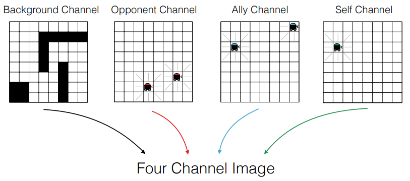
Egorov, M. (2016). Multi-agent deep reinforcement learning., p4.
An important aspect of this data modeling is that by expressing each state of the multi-agent as channels, it is possible to enclose states of all the agents as **a target of convolution operation all at once**. By the affine transformation executed by the neural network, combinations of an enormous number of states of multi-agent can be computed in principle with an allowable range of memory.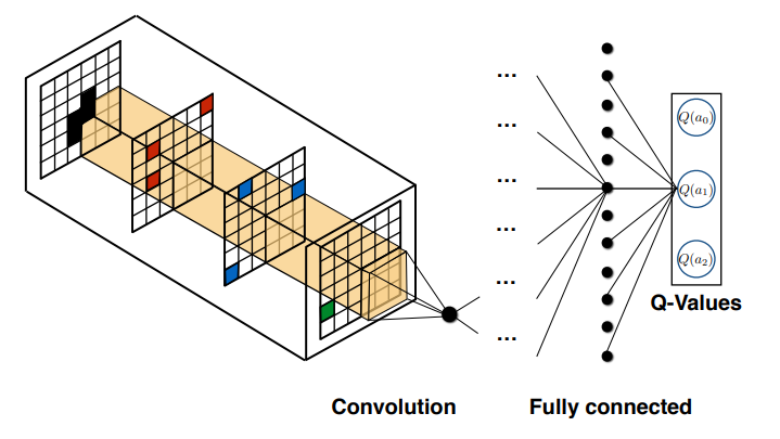
Egorov, M. (2016). Multi-agent deep reinforcement learning., p4.
[demo/multi_agent_maze_by_deep_q_network.ipynb](https://github.com/accel-brain/accel-brain-code/blob/master/Reinforcement-Learning/demo/multi_agent_maze_by_deep_q_network.ipynb) also prototypes Multi Agent Deep Q-Network to solve the pursuit-evasion game based on the image-like state representation of the multi-agent.|
Multi-agent Deep Reinforcement Learning to solve the pursuit-evasion game. The player is caught by enemies. |
Multi-agent Deep Reinforcement Learning to solve the pursuit-evasion game. The player reaches the goal. |
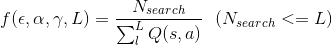
 is the number of searching(learning) and L is a limit of .
Like Monte Carlo method, let us draw random samples from a normal (Gaussian) or unifrom distribution.
```python
# Epsilon-Greedy rate in Epsilon-Greedy-Q-Learning.
greedy_rate_arr = np.random.normal(loc=0.5, scale=0.1, size=100)
# Alpha value in Q-Learning.
alpha_value_arr = np.random.normal(loc=0.5, scale=0.1, size=100)
# Gamma value in Q-Learning.
gamma_value_arr = np.random.normal(loc=0.5, scale=0.1, size=100)
# Limit of the number of Learning(searching).
limit_arr = np.random.normal(loc=10, scale=1, size=100)
var_arr = np.c_[greedy_rate_arr, alpha_value_arr, gamma_value_arr, limit_arr]
```
Instantiate and initialize `MazeGreedyQLearning` which is-a `GreedyQLearning`.
```python
# Instantiation.
greedy_q_learning = MazeGreedyQLearning()
greedy_q_learning.initialize(hoge=fuga)
```
Instantiate `GreedyQLearningCost` which is implemented the interface `CostFunctionable` to be called by `AnnealingModel`.
```python
init_state_key = ("Some", "data")
cost_functionable = GreedyQLearningCost(
greedy_q_learning,
init_state_key=init_state_key
)
```
Instantiate `SimulatedAnnealing` which is-a `AnnealingModel`.
```python
annealing_model = SimulatedAnnealing(
# is-a `CostFunctionable`.
cost_functionable=cost_functionable,
# The number of annealing cycles.
cycles_num=5,
# The number of trials of searching per a cycle.
trials_per_cycle=3
)
```
Fit the `var_arr` to `annealing_model`.
```python
annealing_model.var_arr = var_arr
```
Start annealing.
```python
annealing_model.annealing()
```
To extract result of searching, call the property `predicted_log_list` which is list of tuple: `(Cost, Delta energy, Mean of delta energy, probability in Boltzmann distribution, accept flag)`. And refer the property `x` which is `np.ndarray` that has combination of hyperparameters. The optimal combination can be extracted as follow.
```python
# Extract list: [(Cost, Delta energy, Mean of delta energy, probability, accept)]
predicted_log_arr = annealing_model.predicted_log_arr
# [greedy rate, Alpha value, Gamma value, Limit of the number of searching.]
min_e_v_arr = annealing_model.var_arr[np.argmin(predicted_log_arr[:, 2])]
```
### Contingency of definitions
The above definition of cost function is possible option: not necessity but contingent from the point of view of modal logic. You should questions the necessity of definition and re-define, for designing the implementation of interface `CostFunctionable`, in relation to *your* problem settings.
## Demonstration: Epsilon Greedy Q-Learning and Adaptive Simulated Annealing.
There are various Simulated Annealing such as Boltzmann Annealing, Adaptive Simulated Annealing(SAS), and Quantum Simulated Annealing. On the premise of Combinatorial optimization problem, these annealing methods can be considered as functionally equivalent. The *Commonality/Variability* in these methods are able to keep responsibility of objects all straight as the class diagram below indicates.
is the number of searching(learning) and L is a limit of .
Like Monte Carlo method, let us draw random samples from a normal (Gaussian) or unifrom distribution.
```python
# Epsilon-Greedy rate in Epsilon-Greedy-Q-Learning.
greedy_rate_arr = np.random.normal(loc=0.5, scale=0.1, size=100)
# Alpha value in Q-Learning.
alpha_value_arr = np.random.normal(loc=0.5, scale=0.1, size=100)
# Gamma value in Q-Learning.
gamma_value_arr = np.random.normal(loc=0.5, scale=0.1, size=100)
# Limit of the number of Learning(searching).
limit_arr = np.random.normal(loc=10, scale=1, size=100)
var_arr = np.c_[greedy_rate_arr, alpha_value_arr, gamma_value_arr, limit_arr]
```
Instantiate and initialize `MazeGreedyQLearning` which is-a `GreedyQLearning`.
```python
# Instantiation.
greedy_q_learning = MazeGreedyQLearning()
greedy_q_learning.initialize(hoge=fuga)
```
Instantiate `GreedyQLearningCost` which is implemented the interface `CostFunctionable` to be called by `AnnealingModel`.
```python
init_state_key = ("Some", "data")
cost_functionable = GreedyQLearningCost(
greedy_q_learning,
init_state_key=init_state_key
)
```
Instantiate `SimulatedAnnealing` which is-a `AnnealingModel`.
```python
annealing_model = SimulatedAnnealing(
# is-a `CostFunctionable`.
cost_functionable=cost_functionable,
# The number of annealing cycles.
cycles_num=5,
# The number of trials of searching per a cycle.
trials_per_cycle=3
)
```
Fit the `var_arr` to `annealing_model`.
```python
annealing_model.var_arr = var_arr
```
Start annealing.
```python
annealing_model.annealing()
```
To extract result of searching, call the property `predicted_log_list` which is list of tuple: `(Cost, Delta energy, Mean of delta energy, probability in Boltzmann distribution, accept flag)`. And refer the property `x` which is `np.ndarray` that has combination of hyperparameters. The optimal combination can be extracted as follow.
```python
# Extract list: [(Cost, Delta energy, Mean of delta energy, probability, accept)]
predicted_log_arr = annealing_model.predicted_log_arr
# [greedy rate, Alpha value, Gamma value, Limit of the number of searching.]
min_e_v_arr = annealing_model.var_arr[np.argmin(predicted_log_arr[:, 2])]
```
### Contingency of definitions
The above definition of cost function is possible option: not necessity but contingent from the point of view of modal logic. You should questions the necessity of definition and re-define, for designing the implementation of interface `CostFunctionable`, in relation to *your* problem settings.
## Demonstration: Epsilon Greedy Q-Learning and Adaptive Simulated Annealing.
There are various Simulated Annealing such as Boltzmann Annealing, Adaptive Simulated Annealing(SAS), and Quantum Simulated Annealing. On the premise of Combinatorial optimization problem, these annealing methods can be considered as functionally equivalent. The *Commonality/Variability* in these methods are able to keep responsibility of objects all straight as the class diagram below indicates.
 ### Code sample.
`AdaptiveSimulatedAnnealing` is-a subclass of `SimulatedAnnealing`. The *variability* is aggregated in the method `AdaptiveSimulatedAnnealing.adaptive_set()` which must be called before executing `AdaptiveSimulatedAnnealing.annealing()`.
```python
from pyqlearning.annealingmodel.simulatedannealing.adaptive_simulated_annealing import AdaptiveSimulatedAnnealing
annealing_model = AdaptiveSimulatedAnnealing(
cost_functionable=cost_functionable,
cycles_num=33,
trials_per_cycle=3,
accepted_sol_num=0.0,
init_prob=0.7,
final_prob=0.001,
start_pos=0,
move_range=3
)
# Variability part.
annealing_model.adaptive_set(
# How often will this model reanneals there per cycles.
reannealing_per=50,
# Thermostat.
thermostat=0.,
# The minimum temperature.
t_min=0.001,
# The default temperature.
t_default=1.0
)
annealing_model.var_arr = params_arr
annealing_model.annealing()
```
To extract result of searching, call the property like the case of using `SimulatedAnnealing`. If you want to know how to visualize the searching process, see my Jupyter notebook: [demo/annealing_hand_written_digits.ipynb](https://github.com/chimera0/accel-brain-code/blob/master/Reinforcement-Learning/demo/annealing_hand_written_digits.ipynb).
## Demonstration: Epsilon Greedy Q-Learning and Quantum Monte Carlo.
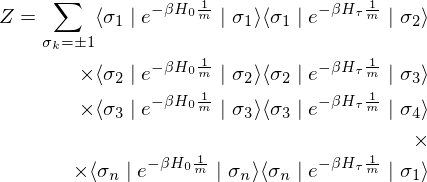
Generally, Quantum Monte Carlo is a stochastic method to solve the Schrödinger equation. This algorithm is one of the earliest types of solution in order to simulate the Quantum Annealing in classical computer. In summary, one of the function of this algorithm is to solve the ground state search problem which is known as logically equivalent to combinatorial optimization problem.
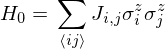
According to theory of spin glasses, the ground state search problem can be described as minimization energy determined by the hamiltonian
### Code sample.
`AdaptiveSimulatedAnnealing` is-a subclass of `SimulatedAnnealing`. The *variability* is aggregated in the method `AdaptiveSimulatedAnnealing.adaptive_set()` which must be called before executing `AdaptiveSimulatedAnnealing.annealing()`.
```python
from pyqlearning.annealingmodel.simulatedannealing.adaptive_simulated_annealing import AdaptiveSimulatedAnnealing
annealing_model = AdaptiveSimulatedAnnealing(
cost_functionable=cost_functionable,
cycles_num=33,
trials_per_cycle=3,
accepted_sol_num=0.0,
init_prob=0.7,
final_prob=0.001,
start_pos=0,
move_range=3
)
# Variability part.
annealing_model.adaptive_set(
# How often will this model reanneals there per cycles.
reannealing_per=50,
# Thermostat.
thermostat=0.,
# The minimum temperature.
t_min=0.001,
# The default temperature.
t_default=1.0
)
annealing_model.var_arr = params_arr
annealing_model.annealing()
```
To extract result of searching, call the property like the case of using `SimulatedAnnealing`. If you want to know how to visualize the searching process, see my Jupyter notebook: [demo/annealing_hand_written_digits.ipynb](https://github.com/chimera0/accel-brain-code/blob/master/Reinforcement-Learning/demo/annealing_hand_written_digits.ipynb).
## Demonstration: Epsilon Greedy Q-Learning and Quantum Monte Carlo.
Generally, Quantum Monte Carlo is a stochastic method to solve the Schrödinger equation. This algorithm is one of the earliest types of solution in order to simulate the Quantum Annealing in classical computer. In summary, one of the function of this algorithm is to solve the ground state search problem which is known as logically equivalent to combinatorial optimization problem.
According to theory of spin glasses, the ground state search problem can be described as minimization energy determined by the hamiltonian  as follow
 where
where  refers to the Pauli spin matrix below for the spin-half particle at lattice point . In spin glasses, random value is assigned to
  . The number of combinations is enormous. If this value is
  , a trial frequency is
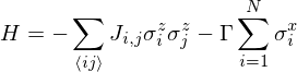
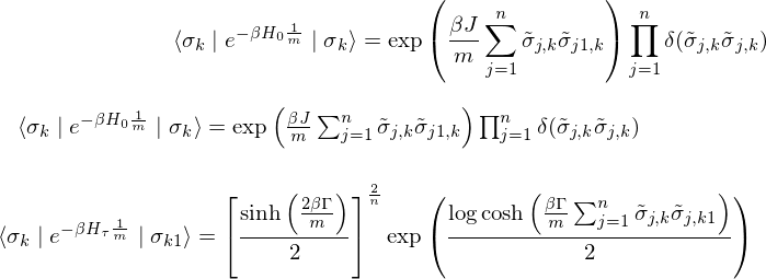
  . This computation complexity makes it impossible to solve the ground state search problem. Then, in theory of spin glasses, the standard hamiltonian is re-described in expanded form.
 where
where  also refers to the Pauli spin matrix and
  is so-called annealing coefficient, which is hyperparameter that contains vely high value. Ising model to follow this Hamiltonian is known as the Transverse Ising model.
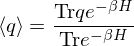
In relation to this system, thermal equilibrium amount of a physical quantity
is so-called annealing coefficient, which is hyperparameter that contains vely high value. Ising model to follow this Hamiltonian is known as the Transverse Ising model.
In relation to this system, thermal equilibrium amount of a physical quantity  is as follow.
 If
If  is a diagonal matrix, then also
  is diagonal matrix. If diagonal element in is
  , Each diagonal element is
  . However if has off-diagonal elements, It is known that
  since for any of the exponent we must exponentiate the matrix as follow.
 Therefore, a path integration based on Trotter-Suzuki decomposition has been introduced in Quantum Monte Carlo Method. This path integration makes it possible to obtain the partition function
  .
.
 where if
  is large enough, relational expression below is established.
 Then the partition function can be re-descibed as follow.
 where
where  is
is  topological products (product spaces). Because is the diagonal matrix,
 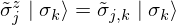 .
Therefore,
.
Therefore,
 The partition function can be re-descibed as follow.
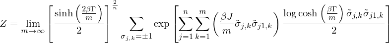 where is the number of trotter.
This relational expression indicates that the quantum - mechanical Hamiltonian in
where is the number of trotter.
This relational expression indicates that the quantum - mechanical Hamiltonian in  dimentional Tranverse Ising model is functional equivalence to classical Hamiltonian in
  dimentional Ising model, which means that the state of the quantum - mechanical system can be approximate by the state of classical system.
### Code sample.
```python
from pyqlearning.annealingmodel.quantum_monte_carlo import QuantumMonteCarlo
from pyqlearning.annealingmodel.distancecomputable.cost_as_distance import CostAsDistance
# User defined function which is-a `CostFuntionable`.
cost_functionable = YourCostFunctions()
# Compute cost as distance for `QuantumMonteCarlo`.
distance_computable = CostAsDistance(params_arr, cost_functionable)
# Init.
annealing_model = QuantumMonteCarlo(
distance_computable=distance_computable,
# The number of annealing cycles.
cycles_num=100,
# Inverse temperature (Beta).
inverse_temperature_beta=0.1,
# Gamma. (so-called annealing coefficient.)
gammma=1.0,
# Attenuation rate for simulated time.
fractional_reduction=0.99,
# The dimention of Trotter.
trotter_dimention=10,
# The number of Monte Carlo steps.
mc_step=100,
# The number of parameters which can be optimized.
point_num=100,
# Default `np.ndarray` of 2-D spin glass in Ising model.
spin_arr=None,
# Tolerance for the optimization.
# When the ΔE is not improving by at least `tolerance_diff_e`
# for two consecutive iterations, annealing will stops.
tolerance_diff_e=0.01
)
# Execute annealing.
annealing_model.annealing()
```
To extract result of searching, call the property like the case of using `SimulatedAnnealing`. If you want to know how to visualize the searching process, see my Jupyter notebook: [demo/annealing_hand_written_digits.ipynb](https://github.com/chimera0/accel-brain-code/blob/master/Reinforcement-Learning/demo/annealing_hand_written_digits.ipynb).
## References
### Q-Learning models.
- Agrawal, S., & Goyal, N. (2011). Analysis of Thompson sampling for the multi-armed bandit problem. arXiv preprint arXiv:1111.1797.
- Bubeck, S., & Cesa-Bianchi, N. (2012). Regret analysis of stochastic and nonstochastic multi-armed bandit problems. arXiv preprint arXiv:1204.5721.
- Chapelle, O., & Li, L. (2011). An empirical evaluation of thompson sampling. In Advances in neural information processing systems (pp. 2249-2257).
- Du, K. L., & Swamy, M. N. S. (2016). Search and optimization by metaheuristics (p. 434). New York City: Springer.
- Kaufmann, E., Cappe, O., & Garivier, A. (2012). On Bayesian upper confidence bounds for bandit problems. In International Conference on Artificial Intelligence and Statistics (pp. 592-600).
- Mnih, V., Kavukcuoglu, K., Silver, D., Graves, A., Antonoglou, I., Wierstra, D., & Riedmiller, M. (2013). Playing atari with deep reinforcement learning. arXiv preprint arXiv:1312.5602.
- Richard Sutton and Andrew Barto (1998). Reinforcement Learning. MIT Press.
- Watkins, C. J. C. H. (1989). Learning from delayed rewards (Doctoral dissertation, University of Cambridge).
- Watkins, C. J., & Dayan, P. (1992). Q-learning. Machine learning, 8(3-4), 279-292.
- White, J. (2012). Bandit algorithms for website optimization. ” O’Reilly Media, Inc.”.
### Deep Q-Network models.
- Cho, K., Van Merriënboer, B., Gulcehre, C., Bahdanau, D., Bougares, F., Schwenk, H., & Bengio, Y. (2014). Learning phrase representations using RNN encoder-decoder for statistical machine translation. arXiv preprint arXiv:1406.1078.
- Egorov, M. (2016). Multi-agent deep reinforcement learning.
- Gupta, J. K., Egorov, M., & Kochenderfer, M. (2017, May). Cooperative multi-agent control using deep reinforcement learning. In International Conference on Autonomous Agents and Multiagent Systems (pp. 66-83). Springer, Cham.
- Malhotra, P., Ramakrishnan, A., Anand, G., Vig, L., Agarwal, P., & Shroff, G. (2016). LSTM-based encoder-decoder for multi-sensor anomaly detection. arXiv preprint arXiv:1607.00148.
- Mnih, V., Kavukcuoglu, K., Silver, D., Graves, A., Antonoglou, I., Wierstra, D., & Riedmiller, M. (2013). Playing atari with deep reinforcement learning. arXiv preprint arXiv:1312.5602.
- Sainath, T. N., Vinyals, O., Senior, A., & Sak, H. (2015, April). Convolutional, long short-term memory, fully connected deep neural networks. In Acoustics, Speech and Signal Processing (ICASSP), 2015 IEEE International Conference on (pp. 4580-4584). IEEE.
- Xingjian, S. H. I., Chen, Z., Wang, H., Yeung, D. Y., Wong, W. K., & Woo, W. C. (2015). Convolutional LSTM network: A machine learning approach for precipitation nowcasting. In Advances in neural information processing systems (pp. 802-810).
- Zaremba, W., Sutskever, I., & Vinyals, O. (2014). Recurrent neural network regularization. arXiv preprint arXiv:1409.2329.
### Annealing models.
- Bektas, T. (2006). The multiple traveling salesman problem: an overview of formulations and solution procedures. Omega, 34(3), 209-219.
- Bertsimas, D., & Tsitsiklis, J. (1993). Simulated annealing. Statistical science, 8(1), 10-15.
- Das, A., & Chakrabarti, B. K. (Eds.). (2005). Quantum annealing and related optimization methods (Vol. 679). Springer Science & Business Media.
- Du, K. L., & Swamy, M. N. S. (2016). Search and optimization by metaheuristics. New York City: Springer.
- Edwards, S. F., & Anderson, P. W. (1975). Theory of spin glasses. Journal of Physics F: Metal Physics, 5(5), 965.
- Facchi, P., & Pascazio, S. (2008). Quantum Zeno dynamics: mathematical and physical aspects. Journal of Physics A: Mathematical and Theoretical, 41(49), 493001.
- Heim, B., Rønnow, T. F., Isakov, S. V., & Troyer, M. (2015). Quantum versus classical annealing of Ising spin glasses. Science, 348(6231), 215-217.
- Heisenberg, W. (1925) Über quantentheoretische Umdeutung kinematischer und mechanischer Beziehungen. Z. Phys. 33, pp.879—893.
- Heisenberg, W. (1927). Über den anschaulichen Inhalt der quantentheoretischen Kinematik und Mechanik. Zeitschrift fur Physik, 43, 172-198.
- Heisenberg, W. (1984). The development of quantum mechanics. In Scientific Review Papers, Talks, and Books -Wissenschaftliche Übersichtsartikel, Vorträge und Bücher (pp. 226-237). Springer Berlin Heidelberg.
Hilgevoord, Jan and Uffink, Jos, "The Uncertainty Principle", The Stanford Encyclopedia of Philosophy (Winter 2016 Edition), Edward N. Zalta (ed.), URL = <https://plato.stanford.edu/archives/win2016/entries/qt-uncertainty/>.
- Jarzynski, C. (1997). Nonequilibrium equality for free energy differences. Physical Review Letters, 78(14), 2690.
- Messiah, A. (1966). Quantum mechanics. 2 (1966). North-Holland Publishing Company.
- Mezard, M., & Montanari, A. (2009). Information, physics, and computation. Oxford University Press.
- Nallusamy, R., Duraiswamy, K., Dhanalaksmi, R., & Parthiban, P. (2009). Optimization of non-linear multiple traveling salesman problem using k-means clustering, shrink wrap algorithm and meta-heuristics. International Journal of Nonlinear Science, 8(4), 480-487.
- Schrödinger, E. (1926). Quantisierung als eigenwertproblem. Annalen der physik, 385(13), S.437-490.
- Somma, R. D., Batista, C. D., & Ortiz, G. (2007). Quantum approach to classical statistical mechanics. Physical review letters, 99(3), 030603.
- 鈴木正. (2008). 「組み合わせ最適化問題と量子アニーリング: 量子断熱発展の理論と性能評価」.,『物性研究』, 90(4): pp598-676. 参照箇所はpp619-624.
- 西森秀稔、大関真之(2018) 『量子アニーリングの基礎』須藤 彰三、岡 真 監修、共立出版、参照箇所はpp9-46.
### More detail demos
- [Webクローラ型人工知能:キメラ・ネットワークの仕様](https://media.accel-brain.com/_chimera-network-is-web-crawling-ai/) (Japanese)
- 20001 bots are running as 20001 web-crawlers and 20001 web-scrapers.
- [ロボアドバイザー型人工知能:キメラ・ネットワークの仕様](https://media.accel-brain.com/_chimera-network-is-robo-adviser/) (Japanese)
- The 20001 bots can also simulate the portfolio optimization of securities such as stocks and circulation currency such as cryptocurrencies.
### Related PoC
- [量子力学、統計力学、熱力学における天才物理学者たちの神学的な形象について](https://accel-brain.com/das-theologische-bild-genialer-physiker-in-der-quantenmechanik-und-der-statistischen-mechanik-und-thermodynamik/) (Japanese)
- [熱力学の前史、マクスウェル=ボルツマン分布におけるエントロピーの歴史的意味論](https://accel-brain.com/das-theologische-bild-genialer-physiker-in-der-quantenmechanik-und-der-statistischen-mechanik-und-thermodynamik/historische-semantik-der-entropie-in-der-maxwell-boltzmann-verteilung/)
- [メディアとしての統計力学と形式としてのアンサンブル、そのギブス的類推](https://accel-brain.com/das-theologische-bild-genialer-physiker-in-der-quantenmechanik-und-der-statistischen-mechanik-und-thermodynamik/statistische-mechanik-als-medium-und-ensemble-als-form/)
- [「マクスウェルの悪魔」、力学の基礎法則としての神](https://accel-brain.com/das-theologische-bild-genialer-physiker-in-der-quantenmechanik-und-der-statistischen-mechanik-und-thermodynamik/maxwell-damon/)
- [Webクローラ型人工知能によるパラドックス探索暴露機能の社会進化論](https://accel-brain.com/social-evolution-of-exploration-and-exposure-of-paradox-by-web-crawling-type-artificial-intelligence/) (Japanese)
- [World-Wide Webの社会構造とWebクローラ型人工知能の意味論](https://accel-brain.com/social-evolution-of-exploration-and-exposure-of-paradox-by-web-crawling-type-artificial-intelligence/sozialstruktur-des-world-wide-web-und-semantik-der-kunstlichen-intelligenz-des-web-crawlers/)
- [意味論の意味論、観察の観察](https://accel-brain.com/social-evolution-of-exploration-and-exposure-of-paradox-by-web-crawling-type-artificial-intelligence/semantik-der-semantik-und-beobachtung-der-beobachtung/)
- [深層強化学習のベイズ主義的な情報探索に駆動された自然言語処理の意味論](https://accel-brain.com/semantics-of-natural-language-processing-driven-by-bayesian-information-search-by-deep-reinforcement-learning/) (Japanese)
- [バンディットアルゴリズムの機能的拡張としての強化学習アルゴリズム](https://accel-brain.com/semantics-of-natural-language-processing-driven-by-bayesian-information-search-by-deep-reinforcement-learning/verstarkungslernalgorithmus-als-funktionale-erweiterung-des-banditenalgorithmus/)
- [深層強化学習の統計的機械学習、強化学習の関数近似器としての深層学習](https://accel-brain.com/semantics-of-natural-language-processing-driven-by-bayesian-information-search-by-deep-reinforcement-learning/deep-learning-als-funktionsapproximator-fur-verstarktes-lernen/)
- [ハッカー倫理に準拠した人工知能のアーキテクチャ設計](https://accel-brain.com/architectural-design-of-artificial-intelligence-conforming-to-hacker-ethics/) (Japanese)
- [アーキテクチャ中心設計の社会構造とアーキテクチャの意味論](https://accel-brain.com/architectural-design-of-artificial-intelligence-conforming-to-hacker-ethics/sozialstruktur-des-architekturzentrum-designs-und-architektur-der-semantik/)
- [「人工の理想」を背景とした「万物照応」のデータモデリング](https://accel-brain.com/data-modeling-von-korrespondenz-in-artificial-paradise/) (Japanese)
- [ギャンブラーの機能的等価物としての強化学習エージェント、投資における冷静沈着な精神の現在性](https://accel-brain.com/data-modeling-von-korrespondenz-in-artificial-paradise/agent-in-reignforcement-lernen-als-funktionelle-aquivalente-von-spielern/)
## Author
- accel-brain
## Author URI
- https://accel-brain.co.jp/
- https://accel-brain.com/
## License
- GNU General Public License v2.0
dimentional Ising model, which means that the state of the quantum - mechanical system can be approximate by the state of classical system.
### Code sample.
```python
from pyqlearning.annealingmodel.quantum_monte_carlo import QuantumMonteCarlo
from pyqlearning.annealingmodel.distancecomputable.cost_as_distance import CostAsDistance
# User defined function which is-a `CostFuntionable`.
cost_functionable = YourCostFunctions()
# Compute cost as distance for `QuantumMonteCarlo`.
distance_computable = CostAsDistance(params_arr, cost_functionable)
# Init.
annealing_model = QuantumMonteCarlo(
distance_computable=distance_computable,
# The number of annealing cycles.
cycles_num=100,
# Inverse temperature (Beta).
inverse_temperature_beta=0.1,
# Gamma. (so-called annealing coefficient.)
gammma=1.0,
# Attenuation rate for simulated time.
fractional_reduction=0.99,
# The dimention of Trotter.
trotter_dimention=10,
# The number of Monte Carlo steps.
mc_step=100,
# The number of parameters which can be optimized.
point_num=100,
# Default `np.ndarray` of 2-D spin glass in Ising model.
spin_arr=None,
# Tolerance for the optimization.
# When the ΔE is not improving by at least `tolerance_diff_e`
# for two consecutive iterations, annealing will stops.
tolerance_diff_e=0.01
)
# Execute annealing.
annealing_model.annealing()
```
To extract result of searching, call the property like the case of using `SimulatedAnnealing`. If you want to know how to visualize the searching process, see my Jupyter notebook: [demo/annealing_hand_written_digits.ipynb](https://github.com/chimera0/accel-brain-code/blob/master/Reinforcement-Learning/demo/annealing_hand_written_digits.ipynb).
## References
### Q-Learning models.
- Agrawal, S., & Goyal, N. (2011). Analysis of Thompson sampling for the multi-armed bandit problem. arXiv preprint arXiv:1111.1797.
- Bubeck, S., & Cesa-Bianchi, N. (2012). Regret analysis of stochastic and nonstochastic multi-armed bandit problems. arXiv preprint arXiv:1204.5721.
- Chapelle, O., & Li, L. (2011). An empirical evaluation of thompson sampling. In Advances in neural information processing systems (pp. 2249-2257).
- Du, K. L., & Swamy, M. N. S. (2016). Search and optimization by metaheuristics (p. 434). New York City: Springer.
- Kaufmann, E., Cappe, O., & Garivier, A. (2012). On Bayesian upper confidence bounds for bandit problems. In International Conference on Artificial Intelligence and Statistics (pp. 592-600).
- Mnih, V., Kavukcuoglu, K., Silver, D., Graves, A., Antonoglou, I., Wierstra, D., & Riedmiller, M. (2013). Playing atari with deep reinforcement learning. arXiv preprint arXiv:1312.5602.
- Richard Sutton and Andrew Barto (1998). Reinforcement Learning. MIT Press.
- Watkins, C. J. C. H. (1989). Learning from delayed rewards (Doctoral dissertation, University of Cambridge).
- Watkins, C. J., & Dayan, P. (1992). Q-learning. Machine learning, 8(3-4), 279-292.
- White, J. (2012). Bandit algorithms for website optimization. ” O’Reilly Media, Inc.”.
### Deep Q-Network models.
- Cho, K., Van Merriënboer, B., Gulcehre, C., Bahdanau, D., Bougares, F., Schwenk, H., & Bengio, Y. (2014). Learning phrase representations using RNN encoder-decoder for statistical machine translation. arXiv preprint arXiv:1406.1078.
- Egorov, M. (2016). Multi-agent deep reinforcement learning.
- Gupta, J. K., Egorov, M., & Kochenderfer, M. (2017, May). Cooperative multi-agent control using deep reinforcement learning. In International Conference on Autonomous Agents and Multiagent Systems (pp. 66-83). Springer, Cham.
- Malhotra, P., Ramakrishnan, A., Anand, G., Vig, L., Agarwal, P., & Shroff, G. (2016). LSTM-based encoder-decoder for multi-sensor anomaly detection. arXiv preprint arXiv:1607.00148.
- Mnih, V., Kavukcuoglu, K., Silver, D., Graves, A., Antonoglou, I., Wierstra, D., & Riedmiller, M. (2013). Playing atari with deep reinforcement learning. arXiv preprint arXiv:1312.5602.
- Sainath, T. N., Vinyals, O., Senior, A., & Sak, H. (2015, April). Convolutional, long short-term memory, fully connected deep neural networks. In Acoustics, Speech and Signal Processing (ICASSP), 2015 IEEE International Conference on (pp. 4580-4584). IEEE.
- Xingjian, S. H. I., Chen, Z., Wang, H., Yeung, D. Y., Wong, W. K., & Woo, W. C. (2015). Convolutional LSTM network: A machine learning approach for precipitation nowcasting. In Advances in neural information processing systems (pp. 802-810).
- Zaremba, W., Sutskever, I., & Vinyals, O. (2014). Recurrent neural network regularization. arXiv preprint arXiv:1409.2329.
### Annealing models.
- Bektas, T. (2006). The multiple traveling salesman problem: an overview of formulations and solution procedures. Omega, 34(3), 209-219.
- Bertsimas, D., & Tsitsiklis, J. (1993). Simulated annealing. Statistical science, 8(1), 10-15.
- Das, A., & Chakrabarti, B. K. (Eds.). (2005). Quantum annealing and related optimization methods (Vol. 679). Springer Science & Business Media.
- Du, K. L., & Swamy, M. N. S. (2016). Search and optimization by metaheuristics. New York City: Springer.
- Edwards, S. F., & Anderson, P. W. (1975). Theory of spin glasses. Journal of Physics F: Metal Physics, 5(5), 965.
- Facchi, P., & Pascazio, S. (2008). Quantum Zeno dynamics: mathematical and physical aspects. Journal of Physics A: Mathematical and Theoretical, 41(49), 493001.
- Heim, B., Rønnow, T. F., Isakov, S. V., & Troyer, M. (2015). Quantum versus classical annealing of Ising spin glasses. Science, 348(6231), 215-217.
- Heisenberg, W. (1925) Über quantentheoretische Umdeutung kinematischer und mechanischer Beziehungen. Z. Phys. 33, pp.879—893.
- Heisenberg, W. (1927). Über den anschaulichen Inhalt der quantentheoretischen Kinematik und Mechanik. Zeitschrift fur Physik, 43, 172-198.
- Heisenberg, W. (1984). The development of quantum mechanics. In Scientific Review Papers, Talks, and Books -Wissenschaftliche Übersichtsartikel, Vorträge und Bücher (pp. 226-237). Springer Berlin Heidelberg.
Hilgevoord, Jan and Uffink, Jos, "The Uncertainty Principle", The Stanford Encyclopedia of Philosophy (Winter 2016 Edition), Edward N. Zalta (ed.), URL = <https://plato.stanford.edu/archives/win2016/entries/qt-uncertainty/>.
- Jarzynski, C. (1997). Nonequilibrium equality for free energy differences. Physical Review Letters, 78(14), 2690.
- Messiah, A. (1966). Quantum mechanics. 2 (1966). North-Holland Publishing Company.
- Mezard, M., & Montanari, A. (2009). Information, physics, and computation. Oxford University Press.
- Nallusamy, R., Duraiswamy, K., Dhanalaksmi, R., & Parthiban, P. (2009). Optimization of non-linear multiple traveling salesman problem using k-means clustering, shrink wrap algorithm and meta-heuristics. International Journal of Nonlinear Science, 8(4), 480-487.
- Schrödinger, E. (1926). Quantisierung als eigenwertproblem. Annalen der physik, 385(13), S.437-490.
- Somma, R. D., Batista, C. D., & Ortiz, G. (2007). Quantum approach to classical statistical mechanics. Physical review letters, 99(3), 030603.
- 鈴木正. (2008). 「組み合わせ最適化問題と量子アニーリング: 量子断熱発展の理論と性能評価」.,『物性研究』, 90(4): pp598-676. 参照箇所はpp619-624.
- 西森秀稔、大関真之(2018) 『量子アニーリングの基礎』須藤 彰三、岡 真 監修、共立出版、参照箇所はpp9-46.
### More detail demos
- [Webクローラ型人工知能:キメラ・ネットワークの仕様](https://media.accel-brain.com/_chimera-network-is-web-crawling-ai/) (Japanese)
- 20001 bots are running as 20001 web-crawlers and 20001 web-scrapers.
- [ロボアドバイザー型人工知能:キメラ・ネットワークの仕様](https://media.accel-brain.com/_chimera-network-is-robo-adviser/) (Japanese)
- The 20001 bots can also simulate the portfolio optimization of securities such as stocks and circulation currency such as cryptocurrencies.
### Related PoC
- [量子力学、統計力学、熱力学における天才物理学者たちの神学的な形象について](https://accel-brain.com/das-theologische-bild-genialer-physiker-in-der-quantenmechanik-und-der-statistischen-mechanik-und-thermodynamik/) (Japanese)
- [熱力学の前史、マクスウェル=ボルツマン分布におけるエントロピーの歴史的意味論](https://accel-brain.com/das-theologische-bild-genialer-physiker-in-der-quantenmechanik-und-der-statistischen-mechanik-und-thermodynamik/historische-semantik-der-entropie-in-der-maxwell-boltzmann-verteilung/)
- [メディアとしての統計力学と形式としてのアンサンブル、そのギブス的類推](https://accel-brain.com/das-theologische-bild-genialer-physiker-in-der-quantenmechanik-und-der-statistischen-mechanik-und-thermodynamik/statistische-mechanik-als-medium-und-ensemble-als-form/)
- [「マクスウェルの悪魔」、力学の基礎法則としての神](https://accel-brain.com/das-theologische-bild-genialer-physiker-in-der-quantenmechanik-und-der-statistischen-mechanik-und-thermodynamik/maxwell-damon/)
- [Webクローラ型人工知能によるパラドックス探索暴露機能の社会進化論](https://accel-brain.com/social-evolution-of-exploration-and-exposure-of-paradox-by-web-crawling-type-artificial-intelligence/) (Japanese)
- [World-Wide Webの社会構造とWebクローラ型人工知能の意味論](https://accel-brain.com/social-evolution-of-exploration-and-exposure-of-paradox-by-web-crawling-type-artificial-intelligence/sozialstruktur-des-world-wide-web-und-semantik-der-kunstlichen-intelligenz-des-web-crawlers/)
- [意味論の意味論、観察の観察](https://accel-brain.com/social-evolution-of-exploration-and-exposure-of-paradox-by-web-crawling-type-artificial-intelligence/semantik-der-semantik-und-beobachtung-der-beobachtung/)
- [深層強化学習のベイズ主義的な情報探索に駆動された自然言語処理の意味論](https://accel-brain.com/semantics-of-natural-language-processing-driven-by-bayesian-information-search-by-deep-reinforcement-learning/) (Japanese)
- [バンディットアルゴリズムの機能的拡張としての強化学習アルゴリズム](https://accel-brain.com/semantics-of-natural-language-processing-driven-by-bayesian-information-search-by-deep-reinforcement-learning/verstarkungslernalgorithmus-als-funktionale-erweiterung-des-banditenalgorithmus/)
- [深層強化学習の統計的機械学習、強化学習の関数近似器としての深層学習](https://accel-brain.com/semantics-of-natural-language-processing-driven-by-bayesian-information-search-by-deep-reinforcement-learning/deep-learning-als-funktionsapproximator-fur-verstarktes-lernen/)
- [ハッカー倫理に準拠した人工知能のアーキテクチャ設計](https://accel-brain.com/architectural-design-of-artificial-intelligence-conforming-to-hacker-ethics/) (Japanese)
- [アーキテクチャ中心設計の社会構造とアーキテクチャの意味論](https://accel-brain.com/architectural-design-of-artificial-intelligence-conforming-to-hacker-ethics/sozialstruktur-des-architekturzentrum-designs-und-architektur-der-semantik/)
- [「人工の理想」を背景とした「万物照応」のデータモデリング](https://accel-brain.com/data-modeling-von-korrespondenz-in-artificial-paradise/) (Japanese)
- [ギャンブラーの機能的等価物としての強化学習エージェント、投資における冷静沈着な精神の現在性](https://accel-brain.com/data-modeling-von-korrespondenz-in-artificial-paradise/agent-in-reignforcement-lernen-als-funktionelle-aquivalente-von-spielern/)
## Author
- accel-brain
## Author URI
- https://accel-brain.co.jp/
- https://accel-brain.com/
## License
- GNU General Public License v2.0