Deep Learning Library: pydbm
pydbm is Python library for building Restricted Boltzmann Machine(RBM), Deep Boltzmann Machine(DBM), Long Short-Term Memory Recurrent Temporal Restricted Boltzmann Machine(LSTM-RTRBM), and Shape Boltzmann Machine(Shape-BM). From the view points of functionally equivalents and structural expansions, this library also prototypes many variants such as Encoder/Decoder based on LSTM with an Attention mechanism, Convolutional Auto-Encoder, ConvLSTM, and Spatio-temporal Auto-Encoder.
pydbm project is dormant. Instead, accel-brain-base project is in progress.
Documentation
Full documentation is available on https://code.accel-brain.com/Deep-Learning-by-means-of-Design-Pattern/ . This document contains information on functionally reusability, functional scalability and functional extensibility.
Installation
Install using pip:
pip install "git+https://github.com/chimera0/accel-brain-code.git#egg=pydbm&subdirectory=Deep-Learning-by-means-of-Design-Pattern"
Or, after cloning this repository, you can install this library with the following command:
git clone https://github.com/chimera0/accel-brain-code.git
cd Deep-Learning-by-means-of-Design-Pattern/
python setup.py bdist_wheel
pip install dist/pydbm-{version}-{hoge}.whl
Source code
The source code is currently hosted on GitHub.
Python package index(PyPI)
Installers for the latest released version are available at the Python package index.
Description
The function of pydbm is building and modeling Restricted Boltzmann Machine(RBM) and Deep Boltzmann Machine(DBM). The models are functionally equivalent to stacked auto-encoder. The basic function is the same as dimensions reduction(or pre-learning). And this library enables you to build many functional extensions from RBM and DBM such as Recurrent Temporal Restricted Boltzmann Machine(RTRBM), Recurrent Neural Network Restricted Boltzmann Machine(RNN-RBM), Long Short-Term Memory Recurrent Temporal Restricted Boltzmann Machine(LSTM-RTRBM), and Shape Boltzmann Machine(Shape-BM).
As more usecases, RTRBM, RNN-RBM, and LSTM-RTRBM can learn dependency structures in temporal patterns such as music, natural sentences, and n-gram. RTRBM is a probabilistic time-series model which can be viewed as a temporal stack of RBMs, where each RBM has a contextual hidden state that is received from the previous RBM and is used to modulate its hidden units bias. The RTRBM can be understood as a sequence of conditional RBMs whose parameters are the output of a deterministic RNN, with the constraint that the hidden units must describe the conditional distributions. This constraint can be lifted by combining a full RNN with distinct hidden units. In terms of this possibility, RNN-RBM and LSTM-RTRBM are structurally expanded model from RTRBM that allows more freedom to describe the temporal dependencies involved.
The usecases of Shape-BM are image segmentation, object detection, inpainting and graphics. Shape-BM is the model for the task of modeling binary shape images, in that samples from the model look realistic and it can generalize to generate samples that differ from training examples.
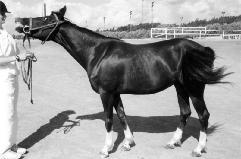
Image in the Weizmann horse dataset. |
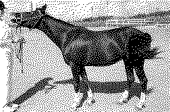
Binarized image. |
Reconstructed image by Shape-BM. |
The structure of RBM.
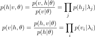
According to graph theory, the structure of RBM corresponds to a complete bipartite graph which is a special kind of bipartite graph where every node in the visible layer is connected to every node in the hidden layer. Based on statistical mechanics and thermodynamics(Ackley, D. H., Hinton, G. E., & Sejnowski, T. J. 1985), the state of this structure can be reflected by the energy function:
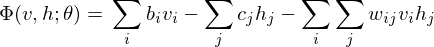
where  is a bias in visible layer,
  is a bias in hidden layer,
  is an activity or a state in visible layer,
  is an activity or a state in hidden layer, and
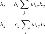
  is a weight matrix in visible and hidden layer. The activities can be calculated as the below product, since the link of activations of visible layer and hidden layer are conditionally independent.
The learning equations of RBM.
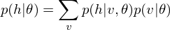
Because of the rules of conditional independence, the learning equations of RBM can be introduced as simple form. The distribution of visible state which is marginalized over the hidden state is as following:

where  is a partition function in statistical mechanics or thermodynamics. Let
  be set of observed data points, then
 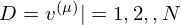 . Therefore the gradients on the parameter
  of the log-likelihood function are
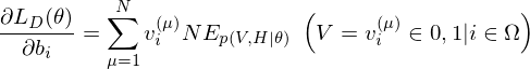


where  is an expected value for
  .
.  is a sigmoid function.
The learning equations of RBM are introduced by performing control so that those gradients can become zero.

Contrastive Divergence as an approximation method.
In relation to RBM, Contrastive Divergence(CD) is a method for approximation of the gradients of the log-likelihood(Hinton, G. E. 2002). The procedure of this method is similar to Markov Chain Monte Carlo method(MCMC). However, unlike MCMC, the visbile variables to be set first in visible layer is not randomly initialized but the observed data points in training dataset are set to the first visbile variables. And, like Gibbs sampler, drawing samples from hidden variables and visible variables is repeated k times. Empirically (and surprisingly), k is considered to be 1.
The structure of DBM.
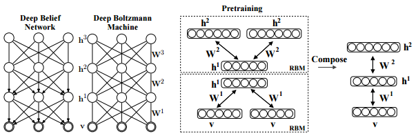
Salakhutdinov, R., Hinton, G. E. (2009). Deep boltzmann machines. In International conference on artificial intelligence and statistics (pp. 448-455). p451.
As is well known, DBM is composed of layers of RBMs stacked on top of each other(Salakhutdinov, R., & Hinton, G. E. 2009). This model is a structural expansion of Deep Belief Networks(DBN), which is known as one of the earliest models of Deep Learning(Le Roux, N., & Bengio, Y. 2008). Like RBM, DBN places nodes in layers. However, only the uppermost layer is composed of undirected edges, and the other consists of directed edges. DBN with R hidden layers is below probabilistic model:
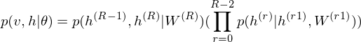
where r = 0 points to visible layer. Considerling simultaneous distribution in top two layer,

and conditional distributions in other layers are as follows:

The pre-learning of DBN engages in a procedure of recursive learning in layer-by-layer. However, as you can see from the difference of graph structure, DBM is slightly different from DBN in the form of pre-learning. For instance, if r = 1, the conditional distribution of visible layer is
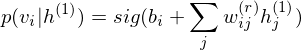 .
.On the other hand, the conditional distribution in the intermediate layer is
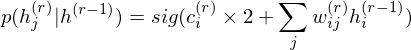
where 2 has been introduced considering that the intermediate layer r receives input data from Shallower layer
r-1 and deeper layer r+1. DBM sets these parameters as initial states.
DBM as a Stacked Auto-Encoder.
DBM is functionally equivalent to a Stacked Auto-Encoder, which is-a neural network that tries to reconstruct its input. To encode the observed data points, the function of DBM is as linear transformation of feature map below
 .
.On the other hand, to decode this feature points, the function of DBM is as linear transformation of feature map below
 .
.The reconstruction error should be calculated in relation to problem setting. This library provides a default method, which can be overridden, for error function that computes Mean Squared Error(MSE). For instance, my jupyter notebook: demo/demo_stacked_auto_encoder.ipynb demonstrates the reconstruction errors of DBM which is a Stacked Auto-Encoder.
Structural expansion for RTRBM.
The RTRBM (Sutskever, I., et al. 2009) is a probabilistic time-series model which can be viewed as a temporal stack of RBMs, where each RBM has a contextual hidden state that is received from the previous RBM and is used to modulate its hidden units bias. Let  be the hidden state in previous step
 t-1. The conditional distribution in hidden layer in time t is

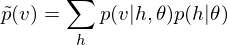
where  is weight matrix in each time steps. Then sampling of observed data points is is as following:

While the hidden units are binary during inference and sampling, it is the mean-field value  that is transmitted to its successors.

Structural expansion for RNN-RBM.
The RTRBM can be understood as a sequence of conditional RBMs whose parameters are the output of a deterministic RNN, with the constraint that the hidden units must describe the conditional distributions and convey temporal information. This constraint can be lifted by combining a full RNN with distinct hidden units. RNN-RBM (Boulanger-Lewandowski, N., et al. 2012), which is the more structural expansion of RTRBM, has also hidden units .
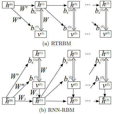
Boulanger-Lewandowski, N., Bengio, Y., & Vincent, P. (2012). Modeling temporal dependencies in high-dimensional sequences: Application to polyphonic music generation and transcription. arXiv preprint arXiv:1206.6392., p4.
Single arrows represent a deterministic function, double arrows represent the stochastic hidden-visible connections of an RBM.
The biases are linear function of . This hidden units are only connected to their direct predecessor  and visible units in time
 t by the relation:

where  and
and  are weight matrixes.
Structural expansion for LSTM-RTRBM.
An example of the application to polyphonic music generation(Lyu, Q., et al. 2015) clued me in on how is it possible to connect RTRBM with LSTM.
Structure of LSTM.
Originally, Long Short-Term Memory(LSTM) networks as a special RNN structure has proven stable and
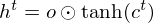
powerful for modeling long-range dependencies. The Key point of structural expansion is its memory cell  which essentially acts as an accumulator of the state information. Every time observed data points are given as new information
  and input to LSTM’s input gate, its information will be accumulated to the cell if the input gate
  is activated. The past state of cell
  could be forgotten in this process if LSTM’s forget gate
  is on. Whether the latest cell output will be propagated to the final state
  is further controlled by the output gate
  .
.
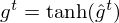
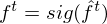
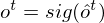
Omitting so-called peephole connection, it makes possible to combine the activations in LSTM gates into an affine transformation below.
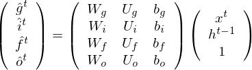
where  is a weight matrix which connects observed data points and hidden units in LSTM gates, and
  is a weight matrix which connects hidden units as a remembered memory in LSTM gates. Furthermore, activation functions are as follows:

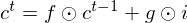
and the acitivation of memory cell and hidden units are calculated as follows:
Structure of LSTM-RTRBM.
LSTM-RTRBM model integrates the ability of LSTM in memorizing and retrieving useful history information, together with the advantage of RBM in high dimensional data modelling(Lyu, Q., Wu, Z., Zhu, J., & Meng, H. 2015, June). Like RTRBM, LSTM-RTRBM also has the recurrent hidden units. Let  be previous hidden units. The conditional distribution of the current hidden layer is as following:

where is a weight matrix which indicates the connectivity between states at each time step in RBM. Now, sampling the observed data points  in RTRBM is as follows.

“Adding LSTM units to RTRBM is not trivial, considering RTRBM’s hidden units and visible units are intertwined in inference and learning. The simplest way to circumvent this difficulty is to use bypass connections from LSTM units to the hidden units besides the existing recurrent connections of hidden units, as in LSTM-RTRBM.”
Therefore it is useful to introduce a distinction of channel which means the sequential information. indicates the direct connectivity in RBM, while  can be defined as a concept representing the previous time step combination in the LSTM units. Let
  and be the hidden units indicating short-term memory and long-term memory, respectively. Then sampling the observed data points in LSTM-RTRBM can be re-described as follows.

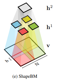
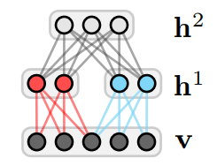
Structural expansion for Shape-BM.
The concept of Shape Boltzmann Machine (Eslami, S. A., et al. 2014) provided inspiration to this library. This model uses below has two layers of hidden variables:  and
and  . The visible units
 v arethe pixels of a binary image of size  . In the visible layer we enforce local receptive fields by connecting each hidden unit in only to a subset of the visible units, corresponding to one of four rectangular patches. In order to encourage boundary consistency each patch overlaps its neighbor by
  pixels and so has side lengths of
  and
and  . In this model, the weight matrix in visible and hidden layer correspond to conectivity between the four sets of hidden units and patches, however the visible biases
  are not shared.
Eslami, S. A., Heess, N., Williams, C. K., & Winn, J. (2014). The shape boltzmann machine: a strong model of object shape. International Journal of Computer Vision, 107(2), 155-176., p156. |
Eslami, S. A., Heess, N., Williams, C. K., & Winn, J. (2014). The shape boltzmann machine: a strong model of object shape. International Journal of Computer Vision, 107(2), 155-176., p156. |
The Shape-BM is a DBM in three layer. The learning algorithm can be completed by optimization of

where 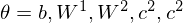 .
.
The Commonality/Variability Analysis in order to practice object-oriented design.
From perspective of commonality/variability analysis in order to practice object-oriented design, the concepts of RBM and DBM paradigms can be organized as follows:

Pay attention to the interface of the above class diagram. While each model is common in that it is constituted by stacked RBM, its approximation methods and activation functions are variable depending on the problem settings.
Considering the commonality, it is useful to design based on Builder Pattern represented by DBMBuilder or RTRBMBuilder, which separates the construction of RBM object RestrictedBoltzmannMachine from its representation by DBMDirector or RTRBMDirector so that the same construction process can create different representations such as DBM, RTRBM, RNN-RBM, and Shape-BM. Additionally, the models of all neural networks are common in that they possess like synapses by obtaining computation graphs without exception. So the class Synapse is contained in various models in a state where computation graphs of weight matrix and bias vector are held in the field.
On the other hand, to deal with the variability, Strategy Pattern, which provides a way to define a family of algorithms such as approximation methods implemented by inheriting the interface ApproximateInterface, and also activation functions implemented by inheriting the interface ActivatingFunctionInterface, is useful design method, which is encapsulate each one as an object, and make them interchangeable from the point of view of functionally equivalent. Template Method Pattern is also useful design method to design the optimizer in this library because this design pattern makes it possible to define the skeleton of an algorithm in a parameter tuning, deferring some steps to client subclasses such as SGD, AdaGrad, RMSProp, NAG, Adam or Nadam. Template Method lets subclasses redefine certain steps of an algorithm without changing the algorithm’s structure.
Functionally equivalent: Encoder/Decoder based on LSTM.
The methodology of equivalent-functionalism enables us to introduce more functional equivalents and compare problem solutions structured with different algorithms and models in common problem setting. For example, in dimension reduction problem, the function of Encoder/Decoder schema is equivalent to DBM as a Stacked Auto-Encoder.
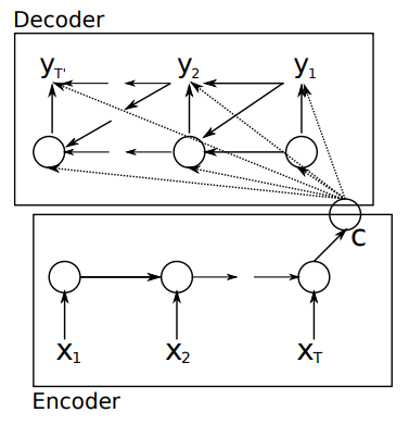
Cho, K., Van Merriënboer, B., Gulcehre, C., Bahdanau, D., Bougares, F., Schwenk, H., & Bengio, Y. (2014). Learning phrase representations using RNN encoder-decoder for statistical machine translation. arXiv preprint arXiv:1406.1078., p2.
According to the neural networks theory, and in relation to manifold hypothesis, it is well known that multilayer neural networks can learn features of observed data points and have the feature points in hidden layer. High-dimensional data can be converted to low-dimensional codes by training the model such as Stacked Auto-Encoder and Encoder/Decoder with a small central layer to reconstruct high-dimensional input vectors. This function of dimensionality reduction facilitates feature expressions to calculate similarity of each data point.
This library provides Encoder/Decoder based on LSTM, which is a reconstruction model and makes it possible to extract series features embedded in deeper layers. The LSTM encoder learns a fixed length vector of time-series observed data points and the LSTM decoder uses this representation to reconstruct the time-series using the current hidden state and the value inferenced at the previous time-step.
As in the above class diagram, in this library, the class EncoderDecoderController can be composed of two LSTMModels. LSTMModel is-a ReconstructableModel, which has a learning method and an inference method like the ordinary supervised learning model.
An example is illustrated in this my jupyter notebook: demo/demo_sine_wave_prediction_by_LSTM_encoder_decoder.ipynb. This notebook demonstrates a simple sine wave prediction by Encoder/Decoder based on LSTM.
Encoder/Decoder for Anomaly Detection(EncDec-AD)
One interesting application example is the Encoder/Decoder for Anomaly Detection (EncDec-AD) paradigm (Malhotra, P., et al. 2016). This reconstruction model learns to reconstruct normal time-series behavior, and thereafter uses reconstruction error to detect anomalies. Malhotra, P., et al. (2016) showed that EncDec-AD paradigm is robust and can detect anomalies from predictable, unpredictable, periodic, aperiodic, and quasi-periodic time-series. Further, they showed that the paradigm is able to detect anomalies from short time-series (length as small as 30) as well as long time-series (length as large as 500).
As the prototype is exemplified in demo/demo_anomaly_detection_by_enc_dec_ad.ipynb, this library provides Encoder/Decoder based on LSTM as a EncDec-AD scheme.
Functionally equivalent: Convolutional Auto-Encoder.
Shape-BM is a kind of problem solution in relation to problem settings such as image segmentation, object detection, inpainting and graphics. In this problem settings, Convolutional Auto-Encoder(Masci, J., et al., 2011) is a functionally equivalent of Shape-BM. A stack of Convolutional Auto-Encoder forms a convolutional neural network(CNN), which are among the most successful models for supervised image classification. Each Convolutional Auto-Encoder is trained using conventional on-line gradient descent without additional regularization terms.
|
Image in the Weizmann horse dataset. |
Reconstructed image by Shape-BM. |
Reconstructed image by Convolutional Auto-Encoder. |
My jupyter notebook: demo/demo_convolutional_auto_encoder.ipynb also demonstrates various reconstructed images.
This library can draw a distinction between Stacked Auto-Encoder and Convolutional Auto-Encoder, and is able to design and implement respective models. Stacked Auto-Encoder ignores the 2 dimentional image structures. In many cases, the rank of observed tensors extracted from image dataset is more than 3. This is not only a problem when dealing with realistically sized inputs, but also introduces redundancy in the parameters, forcing each feature to be global. Like Shape-BM, Convolutional Auto-Encoder differs from Stacked Auto-Encoder as their weights are shared among all locations in the input, preserving spatial locality. Hence, the reconstructed image data is due to a linear combination of basic image patches based on the latent code.
In this library, Convolutional Auto-Encoder is also based on Encoder/Decoder scheme. The encoder is to the decoder what the Convolution is to the Deconvolution. The Deconvolution also called transposed convolutions “work by swapping the forward and backward passes of a convolution.” (Dumoulin, V., & Visin, F. 2016, p20.)
Structural expansion for Convolutional LSTM(ConvLSTM).
Convolutional LSTM(ConvLSTM)(Xingjian, S. H. I. et al., 2015), which is a model that structurally couples convolution operators to LSTM networks, can be utilized as components in constructing the Encoder/Decoder. The ConvLSTM is suitable for spatio-temporal data due to its inherent convolutional structure.
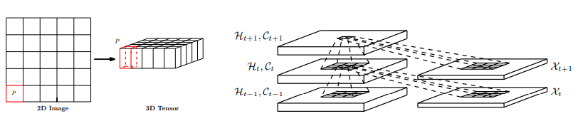
Xingjian, S. H. I., Chen, Z., Wang, H., Yeung, D. Y., Wong, W. K., & Woo, W. C. (2015). Convolutional LSTM network: A machine learning approach for precipitation nowcasting. In Advances in neural information processing systems (pp. 802-810), p806.
This library also makes it possible to build Encoder/Decoder based on ConvLSTM. My jupyter notebook: demo/demo_conv_lstm.ipynb demonstrates that the Encoder/Decoder based on Convolutional LSTM(ConvLSTM) can learn images and reconstruct its.
Structural expansion for Spatio-Temporal Auto-Encoder.
Encoder/Decoder based on ConvLSTM and Convolutional Auto-Encoder have a functional reusability to extend the structures to Spatio-Temporal Auto-Encoder, which can learn the regular patterns in the training videos(Baccouche, M., et al., 2012, Patraucean, V., et al. 2015). This model consists of spatial Auto-Encoder and temporal Encoder/Decoder. The spatial Auto-Encoder is a Convolutional Auto-Encoder for learning spatial structures of each video frame. The temporal Encoder/Decoder is an Encoder/Decoder based on LSTM scheme for learning temporal patterns of the encoded spatial structures. The spatial encoder and decoder have two convolutional and deconvolutional layers respectively, while the temporal encoder and decoder are to act as a twin LSTM models.
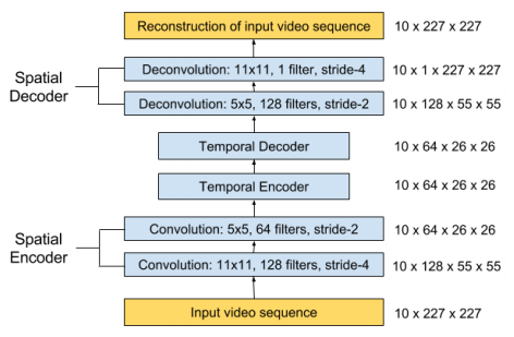
Chong, Y. S., & Tay, Y. H. (2017, June). Abnormal event detection in videos using spatiotemporal autoencoder. In International Symposium on Neural Networks (pp. 189-196). Springer, Cham., p.195.
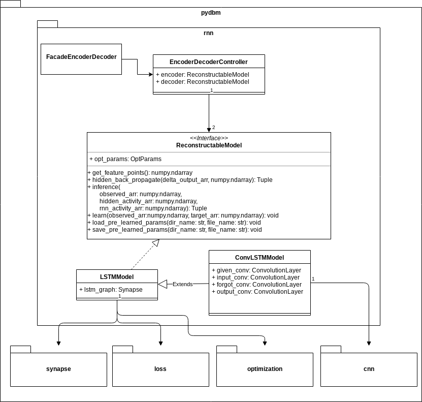
Because of the structural expansions, ConvLSTM and Spatio-Temporal Auto-Encoder can be consisted by cnn subpackage, which is responsible for convolution and deconvolution of spatial features, and rnn subpackage for controlling reconstruction of temporal features as in the following class diagram.
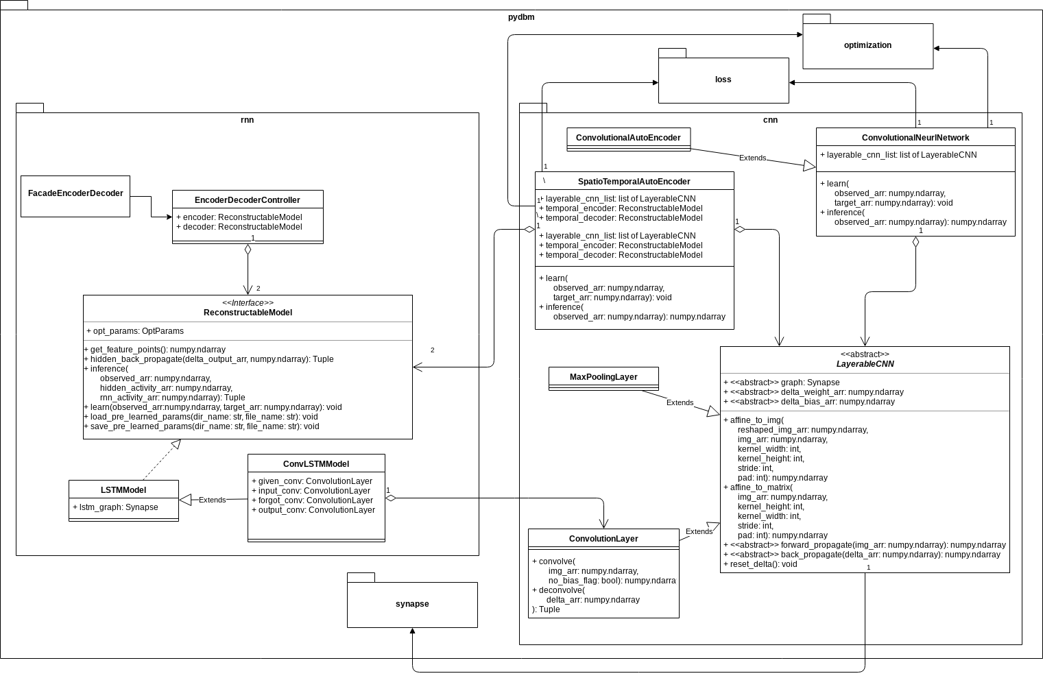
In cnn subpackage, the class LayerableCNN is an abstract class to implement CNN layers such as ConvolutionLayer and MaxPoolingLayer. ConvolutionalAutoEncoder and SpatioTemporalAutoEncoder have those CNN layers, especially ConvolutionLayer to convolve as forward propagation and to deconvolve as back propagation, and are common in the sense that each class has a learning method and an inference method. The difference is that only SpatioTemporalAutoEncoder is related to ReconstructableModel such as LSTMModel and ConvLSTMModel in rnn subpackage.
Video recognition and reconstruction of video images.
demo/demo_spatio_temporal_auto_encoder.ipynb is a jupyter notebook which demonstrates the video recognition and reconstruction of video images by the Spatio-Temporal Auto-Encoder.
Structural extension from Auto-Encoders and Encoder/Decoders to energy-based models and Generative models.
Auto-Encoders, such as the Convolutional Auto-Encoder, the Spatio-Temporal Auto-Encoder, and the DBM have in common that these models are Stacked Auto-Encoders. And the Encoder/Decoder based on LSTM or ConvLSTM share similarity with the RTRBM, RNN-RBM, and LSTM-RTRBM, as the reconstruction models. On the other hand, the Auto-Encoders and the Encoder/Decoders are not statistical mechanical energy-based models unlike with RBM or DBM.
However, Auto-Encoders have traditionally been used to represent energy-based models. According to the statistical mechanical theory for energy-based models, Auto-Encoders constructed by neural networks can be associated with an energy landscape, akin to negative log-probability in a probabilistic model, which measures how well the Auto-Encoder can represent regions in the input space. The energy landscape has been commonly inferred heuristically, by using a training criterion that relates the Auto-Encoder to a probabilistic model such as a RBM. The energy function is identical to the free energy of the corresponding RBM, showing that Auto-Encoders and RBMs may be viewed as two different ways to derive training criteria for forming the same type of analytically defined energy landscape.
The view of the Auto-Encoder as a dynamical system allows us to understand how an energy function may be derived for the Auto-Encoder. This makes it possible to assign energies to Auto-Encoders with many different types of activation functions and outputs, and consider minimanization of reconstruction errors as energy minimanization(Kamyshanska, H., & Memisevic, R., 2014).
When trained with some regularization terms, the Auto-Encoders have the ability to learn an energy manifold without supervision or negative examples(Zhao, J., et al., 2016). This means that even when an energy-based Auto-Encoding model is trained to reconstruct a real sample, the model contributes to discovering the data manifold by itself.
This library provides energy-based Auto-Encoders such as Contractive Convolutional Auto-Encoder(Rifai, S., et al., 2011), Repelling Convolutional Auto-Encoder(Zhao, J., et al., 2016), Denoising Auto-Encoders(Bengio, Y., et al., 2013), and Ladder Networks(Valpola, H., 2015). But it is more usefull to redescribe the Auto-Encoders in the framework of Generative Adversarial Networks(GANs)(Goodfellow, I., et al., 2014) to make those models function as not only energy-based models but also Generative models. For instance, theory of an Adversarial Auto-Encoders(AAEs)(Makhzani, A., et al., 2015) and energy-based GANs(EBGANs)(Zhao, J., et al., 2016) enables us to turn Auto-Encoders into a Generative models which referes energy functions. If you want to implement GANs and AAEs by using pydbm as components for Generative models based on the Statistical machine learning problems, see Generative Adversarial Networks Library: pygan.
Composition and Correspondence in this library
To summarize the information so far into one class diagram, the outline is as follows.
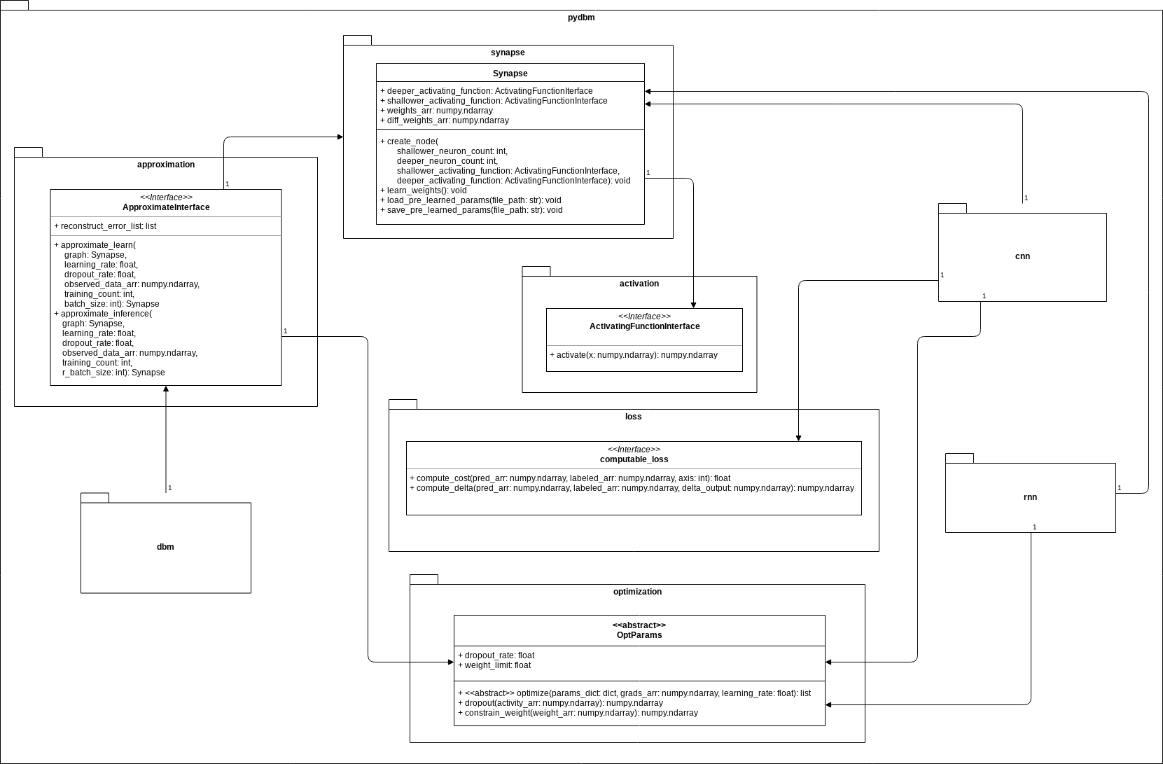
Unlike dbm subpackage, rnn subpackage and cnn subpackage have an association with the interface ComputableLoss. The subclass are Loss functions such as Mean Square Error(MSE) and Cross Entropy. The function of loss functions for dbm is included in the function of energy functions optimized to minimize cost in the interface ApproximateInterface.
Usecase: Building the Deep Boltzmann Machine for feature extracting.
Import Python and Cython modules based on Builder Pattern.
# The `Client` in Builder Pattern
from pydbm.dbm.deep_boltzmann_machine import DeepBoltzmannMachine
# The `Concrete Builder` in Builder Pattern.
from pydbm.dbm.builders.dbm_multi_layer_builder import DBMMultiLayerBuilder
# Contrastive Divergence for function approximation.
from pydbm.approximation.contrastive_divergence import ContrastiveDivergence
Import Python and Cython modules of activation functions.
# Logistic Function as activation function.
from pydbm.activation.logistic_function import LogisticFunction
# Tanh Function as activation function.
from pydbm.activation.tanh_function import TanhFunction
# ReLu Function as activation function.
from pydbm.activation.relu_function import ReLuFunction
Import Python and Cython modules of optimizers, and instantiate the objects.
# Stochastic Gradient Descent(SGD) as optimizer.
from pydbm.optimization.optparams.sgd import SGD

# is-a `OptParams`.
opt_params = SGD(
    # Momentum.
    momentum=0.9
)
If you want to use not Stochastic Gradient Descent(SGD) but Adam(Kingma, D. P., & Ba, J., 2014) optimizer, import Adam and instantiate it.
# Adam as a optimizer.
from pydbm.optimization.optparams.adam import Adam

# is-a `OptParams`.
opt_params = Adam(
    # BETA 1.
    beta_1=0.9,
    # BETA 2.
    beta_2=0.99
)
Setup parameters of regularization. For instance, constraining (or scale down) weight vectors and the probability of dropout(Srivastava, N., Hinton, G., et al., 2014, Zaremba, W., et al., 2014) can be set as follows.
# Regularization for weights matrix
# to repeat multiplying the weights matrix and `0.9`
# until $\sum_{j=0}^{n}w_{ji}^2 < weight\_limit$.
opt_params.weight_limit = 1e+03

# Probability of dropout.
opt_params.dropout_rate = 0.5
Instantiate objects and call the method.
# Contrastive Divergence for visible layer and first hidden layer.
first_cd = ContrastiveDivergence(opt_params=opt_params)
# Contrastive Divergence for first hidden layer and second hidden layer.
second_cd = ContrastiveDivergence(opt_params=opt_params)

# DBM
dbm = DeepBoltzmannMachine(
    # `Concrete Builder` in Builder Pattern,
    # which composes three restricted boltzmann machines for building a deep boltzmann machine.
    DBMMultiLayerBuilder(),
    # Dimention in visible layer, hidden layer, and second hidden layer.
    [train_arr.shape[1], 10, train_arr.shape[1]],
    # Setting objects for activation function.
    [ReLuFunction(), LogisticFunction(), TanhFunction()],
    # Setting the object for function approximation.
    [first_cd, second_cd],
    # Setting learning rate.
    learning_rate=0.05
)

# Execute learning.
dbm.learn(
    # `np.ndarray` of observed data points.
    train_arr,
     # If approximation is the Contrastive Divergence, this parameter is `k` in CD method.
    training_count=1,
    # Batch size in mini-batch training.
    batch_size=200,
    # if `r_batch_size` > 0, the function of `dbm.learn` is a kind of reccursive learning.
    r_batch_size=-1
)
If you do not want to execute the mini-batch training, the value of batch_size must be -1. And r_batch_size is also parameter to control the mini-batch training but is refered only in inference and reconstruction. If this value is more than 0, the inferencing is a kind of reccursive learning with the mini-batch training.
And the feature points can be extracted by this method.
feature_point_arr = dbm.get_feature_point(layer_number=1)
Usecase: Extracting all feature points for dimensions reduction(or pre-learning)
Import Python and Cython modules and instantiate the objects in the same manner as Usecase: Building the Deep Boltzmann Machine for feature extracting.
Import and instantiate not DeepBoltzmannMachine but StackedAutoEncoder, and call the method.
# `StackedAutoEncoder` is-a `DeepBoltzmannMachine`.
from pydbm.dbm.deepboltzmannmachine.stacked_auto_encoder import StackedAutoEncoder

# is-a `DeepBoltzmannMachine`.
dbm = StackedAutoEncoder(
    DBMMultiLayerBuilder(),
    [target_arr.shape[1], 10, target_arr.shape[1]],
    activation_list,
    approximaion_list,
    learning_rate=0.05 # Setting learning rate.
)

# Execute learning.
dbm.learn(
    target_arr,
    1, # If approximation is the Contrastive Divergence, this parameter is `k` in CD method.
    batch_size=200,  # Batch size in mini-batch training.
    r_batch_size=-1  # if `r_batch_size` > 0, the function of `dbm.learn` is a kind of reccursive learning.
)
The function of computable_loss is computing the reconstruction error. MeanSquaredError is-a ComputableLoss, which is so-called Loss function.
Extract reconstruction error rate.
You can check the reconstruction error rate. During the approximation of the Contrastive Divergence, the mean squared error(MSE) between the observed data points and the activities in visible layer is computed as the reconstruction error rate.
Call get_reconstruct_error_arr method as follow.
reconstruct_error_arr = dbm.get_reconstruct_error_arr(layer_number=0)
layer_number corresponds to the index of approximaion_list. And reconstruct_error_arr is the np.ndarray of reconstruction error rates.
Extract the result of dimention reduction
And the result of dimention reduction can be extracted by this property.
pre_learned_arr = dbm.feature_points_arr
Extract weights obtained by pre-learning.
If you want to get the pre-learning weights, call get_weight_arr_list method.
weight_arr_list = dbm.get_weight_arr_list()
weight_arr_list is the list of weights of each links in DBM. weight_arr_list[0] is 2-d np.ndarray of weights between visible layer and first hidden layer.
Extract biases obtained by pre-learning.
Call get_visible_bias_arr_list method and get_hidden_bias_arr_list method in the same way.
visible_bias_arr_list = dbm.get_visible_bias_arr_list()
hidden_bias_arr_list = dbm.get_hidden_bias_arr_list()
visible_bias_arr_list and hidden_bias_arr_list are the list of biases of each links in DBM.
Save pre-learned parameters.
The object dbm, which is-a DeepBoltzmannMachine, has the method save_pre_learned_params, to store the pre-learned parameters in compressed NPY format files.
# Save pre-learned parameters.
dbm.save_pre_learned_params(
    # Path of dir. If `None`, the file is saved in the current directory.
    dir_path="/var/tmp/",
    # The naming rule of files. If `None`, this value is `dbm`.
    file_name="demo_dbm"
)
Transfer learning in DBM.
DBMMultiLayerBuilder can be given pre_learned_path_list which is a list of file paths that store pre-learned parameters.
dbm = StackedAutoEncoder(
    DBMMultiLayerBuilder(
        # `list` of file path that stores pre-learned parameters.
        pre_learned_path_list=[
            "/var/tmp/demo_dbm_0.npz",
            "/var/tmp/demo_dbm_1.npz"
        ]
    ),
    [next_target_arr.shape[1], 10, next_target_arr.shape[1]],
    activation_list,
    approximaion_list,
    # Setting learning rate.
    0.05
)

# Execute learning.
dbm.learn(
    next_target_arr,
    1, # If approximation is the Contrastive Divergence, this parameter is `k` in CD method.
    batch_size=200,  # Batch size in mini-batch training.
    r_batch_size=-1  # if `r_batch_size` > 0, the function of `dbm.learn` is a kind of reccursive learning.
)
If you want to know how to minimize the reconstructed error, see my Jupyter notebook: demo/demo_stacked_auto_encoder.ipynb.
Performance
Run a program: test/demo_stacked_auto_encoder.py
time python test/demo_stacked_auto_encoder.py
The result is follow.
real    1m59.875s
user    1m30.642s
sys     0m29.232s
Detail
This experiment was performed under the following conditions.
Machine type
- vCPU:
2 - memory:
8GB - CPU Platform: Intel Ivy Bridge
Observation Data Points
The observated data is the result of np.random.normal(loc=0.5, scale=0.2, size=(10000, 10000)).
Number of units
- Visible layer:
10000 - hidden layer(feature point):
10 - hidden layer:
10000
Activation functions
- visible: Logistic Function
- hidden(feature point): Logistic Function
- hidden: Logistic Function
Approximation
- Contrastive Divergence
Hyper parameters
- Learning rate:
0.05 - Dropout rate:
0.5
Feature points
[[0.092057   0.08856277 0.08699257 ... 0.09167331 0.08937846 0.0880063 ]
 [0.09090537 0.08669612 0.08995347 ... 0.08641837 0.08750935 0.08617442]
 [0.10187259 0.10633451 0.10060372 ... 0.10170306 0.10711189 0.10565192]
 ...
 [0.21540273 0.21737737 0.20949192 ... 0.20974982 0.2208562  0.20894371]
 [0.30749327 0.30964707 0.2850683  ... 0.29191507 0.29968456 0.29075691]
 [0.68022984 0.68454348 0.66431651 ... 0.67952715 0.6805653  0.66243178]]
Usecase: Building the RTRBM for recursive learning.
Import Python and Cython modules.
# Logistic Function as activation function.
from pydbm.activation.logistic_function import LogisticFunction
# Tanh Function as activation function.
from pydbm.activation.tanh_function import TanhFunction
# Stochastic Gradient Descent(SGD) as optimizer.
from pydbm.optimization.optparams.sgd import SGD
# The `Client` in Builder Pattern for building RTRBM.
from pydbm.dbm.recurrent_temporal_rbm import RecurrentTemporalRBM
Instantiate objects and execute learning.
# The `Client` in Builder Pattern for building RTRBM.
rt_rbm = RecurrentTemporalRBM(
    # The number of units in visible layer.
    visible_num=observed_arr.shape[-1],
    # The number of units in hidden layer.
    hidden_num=100,
    # The activation function in visible layer.
    visible_activating_function=TanhFunction(),
    # The activation function in hidden layer.
    hidden_activating_function=TanhFunction(),
    # The activation function in RNN layer.
    rnn_activating_function=LogisticFunction(),
    # is-a `OptParams`.
    opt_params=SGD(),
    # Learning rate.
    learning_rate=1e-05
)
Learning.
The rt_rbm has a learn method, to execute learning observed data points. This method can receive a np.ndarray of observed data points, which is a rank-3 array-like or sparse matrix of shape: (The number of samples, The length of cycle, The number of features), as the first argument.
# Learning.
rt_rbm.learn(
    # The `np.ndarray` of observed data points.
    observed_arr,
    # Training count.
    training_count=1000,
    # Batch size.
    batch_size=200
)
Inferencing.
After learning, the rt_rbm provides a function of inference method.
# Execute recursive learning.
inferenced_arr = rt_rbm.inference(
    test_arr,
    training_count=1,
    r_batch_size=-1
)
The shape of test_arr is equivalent to observed_arr. Returned value inferenced_arr is generated by input parameter test_arr and can be considered as a feature expression of test_arr based on the distribution of observed_arr. In other words, the features of inferenced_arr is a summary of time series information in test_arr and then the shape is rank-2 array-like or sparse matrix: (The number of samples, The number of features).
Feature points.
On the other hand, the rt_rbm has a rbm which also stores the feature points in hidden layers. To extract this embedded data, call the method as follows.
feature_points_arr = rt_rbm.rbm.get_feature_points()
The shape of feature_points_arr is rank-2 array-like or sparse matrix: (The number of samples, The number of units in hidden layers). So this matrix also means time series data embedded as manifolds.
Reconstructed data.
Although RTRBM itself is not an Auto-Encoder, it can be described as a reconstruction model. In this library, this model has an input reconstruction function.
reconstructed_arr = rt_rbm.rbm.get_reconstructed_arr()
The shape of reconstructed_arr is equivalent to observed_arr.
If you want to know how to measure its reconstruction errors, see my Jupyter notebook: demo/demo_rt_rbm.ipynb.
Save pre-learned parameters.
The object rt_rbm, which is-a RecurrentTemporalRBM, has the method save_pre_learned_params, to store the pre-learned parameters in a compressed NPY format file.
rt_rbm.save_pre_learned_params("/var/tmp/demo_rtrbm.npz")
Transfer learning in RTRBM.
__init__ method of RecurrentTemporalRBM can be given pre_learned_path_list which is a str of file path that stores pre-learned parameters.
# The `Client` in Builder Pattern for building RTRBM.
rt_rbm = RecurrentTemporalRBM(
    # The number of units in visible layer.
    visible_num=observed_arr.shape[-1],
    # The number of units in hidden layer.
    hidden_num=100,
    # The activation function in visible layer.
    visible_activating_function=TanhFunction(),
    # The activation function in hidden layer.
    hidden_activating_function=TanhFunction(),
    # The activation function in RNN layer.
    rnn_activating_function=LogisticFunction(),
    # is-a `OptParams`.
    opt_params=SGD(),
    # Learning rate.
    learning_rate=1e-05,
    # File path that stores pre-learned parameters.
    pre_learned_path="/var/tmp/demo_rtrbm.npz"
)

# Learning.
rt_rbm.learn(
    # The `np.ndarray` of observed data points.
    observed_arr,
    # Training count.
    training_count=1000,
    # Batch size.
    batch_size=200
)
Usecase: Building the RNN-RBM for recursive learning.
Import not RecurrentTemporalRBM but RNNRBM, which is-a RecurrentTemporalRBM.
# The `Client` in Builder Pattern for building RNN-RBM.
from pydbm.dbm.recurrenttemporalrbm.rnn_rbm import RNNRBM
Instantiate objects.
# The `Client` in Builder Pattern for building RNN-RBM.
rt_rbm = RNNRBM(
    # The number of units in visible layer.
    visible_num=observed_arr.shape[-1],
    # The number of units in hidden layer.
    hidden_num=100,
    # The activation function in visible layer.
    visible_activating_function=TanhFunction(),
    # The activation function in hidden layer.
    hidden_activating_function=TanhFunction(),
    # The activation function in RNN layer.
    rnn_activating_function=LogisticFunction(),
    # is-a `OptParams`.
    opt_params=SGD(),
    # Learning rate.
    learning_rate=1e-05
)
The function of learning, inferencing, saving pre-learned parameters, and transfer learning are equivalent to rt_rbm of RTRBM. See Usecase: Building the RTRBM for recursive learning..
If you want to know how to measure its reconstruction errors, see my Jupyter notebook: demo/demo_rnn_rbm.ipynb.
Usecase: Building the LSTM-RTRBM for recursive learning.
Import not RecurrentTemporalRBM but LSTMRTRBM, which is-a RecurrentTemporalRBM.
# The `Client` in Builder Pattern for building LSTM-RTRBM.
from pydbm.dbm.recurrenttemporalrbm.lstm_rt_rbm import LSTMRTRBM
Instantiate objects.
# The `Client` in Builder Pattern for building RNN-RBM.
rt_rbm = LSTMRTRBM(
    # The number of units in visible layer.
    visible_num=observed_arr.shape[-1],
    # The number of units in hidden layer.
    hidden_num=100,
    # The activation function in visible layer.
    visible_activating_function=TanhFunction(),
    # The activation function in hidden layer.
    hidden_activating_function=TanhFunction(),
    # The activation function in RNN layer.
    rnn_activating_function=LogisticFunction(),
    # is-a `OptParams`.
    opt_params=SGD(),
    # Learning rate.
    learning_rate=1e-05
)
The function of learning, inferencing, saving pre-learned parameters, and transfer learning are equivalent to rt_rbm of RTRBM. See Usecase: Building the RTRBM for recursive learning..
If you want to know how to measure its reconstruction errors, see my Jupyter notebook: demo/demo_lstm_rt_rbm.ipynb.
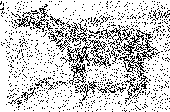
Usecase: Image segmentation by Shape-BM.
First, acquire image data and binarize it.
from PIL import Image
img = Image.open("horse099.jpg")
img
If you think the size of your image datasets may be large, resize it to an arbitrary size.
img = img.resize((255, 255))
Convert RGB images to binary images.
img_bin = img.convert("1")
img_bin
Set up hyperparameters.
filter_size = 5
overlap_n = 4

learning_rate = 0.01
filter_size is the ‘filter’ size. This value must be more than 4. And overlap_n is hyperparameter specific to Shape-BM. In the visible layer, this model has so-called local receptive fields by connecting each first hidden unit only to a subset of the visible units, corresponding to one of four square patches. Each patch overlaps its neighbor by overlap_n pixels (Eslami, S. A., et al, 2014).
Please note that the recommended ratio of filter_size and overlap_n is 5:4. It is not a constraint demanded by pure theory of Shape Boltzmann Machine itself but is a kind of limitation to simplify design and implementation in this library.
And import Python and Cython modules.
# The `Client` in Builder Pattern
from pydbm.dbm.deepboltzmannmachine.shape_boltzmann_machine import ShapeBoltzmannMachine
# The `Concrete Builder` in Builder Pattern.
from pydbm.dbm.builders.dbm_multi_layer_builder import DBMMultiLayerBuilder
Instantiate objects and call the method.
dbm = ShapeBoltzmannMachine(
    DBMMultiLayerBuilder(),
    learning_rate=learning_rate,
    overlap_n=overlap_n,
    filter_size=filter_size
)

img_arr = np.asarray(img_bin)
img_arr = img_arr.astype(np.float64)

# Execute learning.
dbm.learn(
    # `np.ndarray` of image data.
    img_arr,
    # If approximation is the Contrastive Divergence, this parameter is `k` in CD method.
    training_count=1,
    # Batch size in mini-batch training.
    batch_size=300,
    # if `r_batch_size` > 0, the function of `dbm.learn` is a kind of reccursive learning.
    r_batch_size=-1,
    # Learning with the stochastic gradient descent(SGD) or not.
    sgd_flag=True
)
Extract dbm.visible_points_arr as the observed data points in visible layer. This np.ndarray is segmented image data.
inferenced_data_arr = dbm.visible_points_arr.copy()
inferenced_data_arr = 255 - inferenced_data_arr
Image.fromarray(np.uint8(inferenced_data_arr))
Save pre-learned parameters and transfer learning in Shape Boltzmann Machine.
In transfer learning problem setting, ShapeBoltzmannMachine is functionally equivalent to StackedAutoEncoder. See Usecase: Extracting all feature points for dimensions reduction(or pre-learning).
Usecase: Casual use by facade for building Encoder/Decoder based on LSTM.
Import facade module for building Encoder/Decoder based on LSTM.
from pydbm.rnn.facade_encoder_decoder import FacadeEncoderDecoder
If you want to use an Attention mechanism, import FacadeAttentionEncoderDecoder instead.
from pydbm.rnn.facade_attention_encoder_decoder import FacadeAttentionEncoderDecoder as FacadeEncoderDecoder
Instantiate object and call the method to learn observed data points.
# `Facade` for casual user of Encoder/Decoder based on LSTM networks.
facade_encoder_decoder = FacadeEncoderDecoder(
    # The number of units in input layers.
    input_neuron_count=observed_arr.shape[-1],
    # The length of sequences.
    # This means refereed maxinum step `t` in feedforward.
    seq_len=observed_arr.shape[1],
    # Refereed maxinum step `t` in BPTT. If `0`, this class referes all past data in BPTT.
    bptt_tau=observed_arr.shape[1],
    # Verbose mode or not. If `True`, this class sets the logger level as `DEBUG`.
    verbose_flag=True
)
Execute learning.
facade_encoder_decoder.learn(
    observed_arr=observed_arr,
    target_arr=observed_arr
)
This method can receive a np.ndarray of observed data points, which is a rank-3 array-like or sparse matrix of shape: (The number of samples, The length of cycle, The number of features), as the first and second argument. If the value of this second argument is not equivalent to the first argument and the shape is (The number of samples, The number of features), in other words, the rank is 2, the function of encoder_decoder_controller corresponds to a kind of Regression model.
After learning, the facade_encoder_decoder provides a function of inference method.
# Execute recursive learning.
inferenced_arr = facade_encoder_decoder.inference(test_arr)
The shape of test_arr and inferenced_arr are equivalent to observed_arr. Returned value inferenced_arr is generated by input parameter test_arr and can be considered as a decoded data points based on encoded test_arr.
On the other hand, the facade_encoder_decoder also stores the feature points in hidden layers. To extract this embedded data, call the method as follows.
feature_points_arr = facade_encoder_decoder.get_feature_points()
The shape of feature_points_arr is rank-2 array-like or sparse matrix: (The number of samples, The number of units in hidden layers). So this matrix also means time series data embedded as manifolds.
You can check the reconstruction error rate. Call get_reconstruct_error method as follow.
reconstruct_error_arr = facade_encoder_decoder.get_reconstruction_error()
If you want to know how to minimize the reconstructed error, see my Jupyter notebook: demo/demo_sine_wave_prediction_by_LSTM_encoder_decoder.ipynb.
Save pre-learned parameters.
The object facade_encoder_decoder has the method save_pre_learned_params, to store the pre-learned parameters in compressed NPY format files.
facade_encoder_decoder.save_pre_learned_params(
    # File path that stores Encoder's parameters.
    encoder_file_path="/var/tmp/encoder.npz",
    # File path that stores Decoder's parameters.
    decoder_file_path="/var/tmp/decoder.npz"
)
Transfer learning in Encoder/Decoder based on LSTM.
__init__ method of FacadeEncoderDecoder can be given encoder_pre_learned_file_path and decoder_pre_learned_file_path, which are str of file path that stores Encoder/Decoder’s pre-learned parameters.
facade_encoder_decoder2 = FacadeEncoderDecoder(
    # The number of units in input layers.
    input_neuron_count=observed_arr.shape[-1],
    # The length of sequences.
    # This means refereed maxinum step `t` in feedforward.
    seq_len=observed_arr.shape[1],
    # Refereed maxinum step `t` in BPTT. If `0`, this class referes all past data in BPTT.
    bptt_tau=observed_arr.shape[1],
    # File path that stored Encoder's pre-learned parameters.
    encoder_pre_learned_file_path="/var/tmp/encoder.npz",
    # File path that stored Decoder's pre-learned parameters.
    decoder_pre_learned_file_path="/var/tmp/decoder.npz",
    # Verbose mode or not. If `True`, this class sets the logger level as `DEBUG`.
    verbose_flag=True
)

facade_encoder_decoder2.learn(
    observed_arr=observed_arr,
    target_arr=observed_arr
)
For more detail settings.
__init__ of FacadeEncoderDecoder can be given many parameters as follows.
# `Facade` for casual user of Encoder/Decoder based on LSTM networks.
facade_encoder_decoder = FacadeEncoderDecoder(
    # The number of units in input layers.
    input_neuron_count=observed_arr.shape[-1],
    # The number of units in hidden layers.
    hidden_neuron_count=200,
    # Epochs of Mini-batch.
    epochs=200,
    # Batch size of Mini-batch.
    batch_size=20,
    # Learning rate.
    learning_rate=1e-05,
    # Attenuate the `learning_rate` by a factor of this value every `attenuate_epoch`.
    learning_attenuate_rate=0.1,
    # Attenuate the `learning_rate` by a factor of `learning_attenuate_rate` every `attenuate_epoch`.
    attenuate_epoch=50,
    # Activation function in hidden layers.
    hidden_activating_function=LogisticFunction(),
    # Activation function in output layers.
    output_activating_function=LogisticFunction(),
    # Loss function.
    computable_loss=MeanSquaredError(),
    # Optimizer which is-a `OptParams`.
    opt_params=Adam(),
    # The length of sequences.
    # This means refereed maxinum step `t` in feedforward.
    seq_len=8,
    # Refereed maxinum step `t` in Backpropagation Through Time(BPTT).
    # If `0`, this class referes all past data in BPTT.
    bptt_tau=8,
    # Size of Test data set. If this value is `0`, the validation will not be executed.
    test_size_rate=0.3,
    # Tolerance for the optimization.
    # When the loss or score is not improving by at least tol
    # for two consecutive iterations, convergence is considered
    # to be reached and training stops.
    tol=0.0,
    # Tolerance for deviation of loss.
    tld=1.0,
    # Verification function.
    verificatable_result=VerificateFunctionApproximation(),
    # Verbose mode or not. If `True`, this class sets the logger level as `DEBUG`.
    verbose_flag=True
)
If you want to not only use casually the model but also hack it, see Usecase: Build Encoder/Decoder based on LSTM as a reconstruction model..
Usecase: Build Encoder/Decoder based on LSTM or ConvLSTM as a reconstruction model.
Consider functionally reusability and possibility of flexible design, you should use not FacadeEncoderDecoder but EncoderDecoderController as follows.
Setup logger for verbose output.
from logging import getLogger, StreamHandler, NullHandler, DEBUG, ERROR

logger = getLogger("pydbm")
handler = StreamHandler()
handler.setLevel(DEBUG)
logger.setLevel(DEBUG)
logger.addHandler(handler)
Import Python and Cython modules for computation graphs.
# LSTM Graph which is-a `Synapse`.
from pydbm.synapse.recurrenttemporalgraph.lstm_graph import LSTMGraph as EncoderGraph
from pydbm.synapse.recurrenttemporalgraph.lstm_graph import LSTMGraph as DecoderGraph
If you want to introduce the graph of decoder for building an Attention mechanism as the decoder, import AttentionLSTMGraph instead.
from pydbm.synapse.recurrenttemporalgraph.lstmgraph.attention_lstm_graph import AttentionLSTMGraph as DecoderGraph
Import Python and Cython modules of activation functions.
# Logistic Function as activation function.
from pydbm.activation.logistic_function import LogisticFunction
# Tanh Function as activation function.
from pydbm.activation.tanh_function import TanhFunction
Import Python and Cython modules for loss function.
# Loss function.
from pydbm.loss.mean_squared_error import MeanSquaredError
Import Python and Cython modules for optimizer.
# SGD as a optimizer.
from pydbm.optimization.optparams.sgd import SGD as EncoderSGD
from pydbm.optimization.optparams.sgd import SGD as DecoderSGD
If you want to use not Stochastic Gradient Descent(SGD) but Adam optimizer, import Adam.
# Adam as a optimizer.
from pydbm.optimization.optparams.adam import Adam as EncoderAdam
from pydbm.optimization.optparams.adam import Adam as DecoderAdam
Futhermore, import class for verification of function approximation.
# Verification.
from pydbm.verification.verificate_function_approximation import VerificateFunctionApproximation
The activation by softmax function can be verificated by VerificateSoftmax.
from pydbm.verification.verificate_softmax import VerificateSoftmax
And import LSTM Model and Encoder/Decoder schema.
# LSTM model.
from pydbm.rnn.lstm_model import LSTMModel as Encoder
from pydbm.rnn.lstm_model import LSTMModel as Decoder

# Encoder/Decoder
from pydbm.rnn.encoder_decoder_controller import EncoderDecoderController
If you want to build an Attention mechanism as the decoder, import AttentionLSTMModel instead.
from pydbm.rnn.lstmmodel.attention_lstm_model import AttentionLSTMModel as Decoder
Instantiate Encoder.
# Init.
encoder_graph = EncoderGraph()

# Activation function in LSTM.
encoder_graph.observed_activating_function = TanhFunction()
encoder_graph.input_gate_activating_function = LogisticFunction()
encoder_graph.forget_gate_activating_function = LogisticFunction()
encoder_graph.output_gate_activating_function = LogisticFunction()
encoder_graph.hidden_activating_function = TanhFunction()
encoder_graph.output_activating_function = LogisticFunction()

# Initialization strategy.
# This method initialize each weight matrices and biases in Gaussian distribution: `np.random.normal(size=hoge) * 0.01`.
encoder_graph.create_rnn_cells(
    input_neuron_count=observed_arr.shape[-1],
    hidden_neuron_count=200,
    output_neuron_count=1
)

# Optimizer for Encoder.
encoder_opt_params = EncoderAdam()
encoder_opt_params.weight_limit = 1e+03
encoder_opt_params.dropout_rate = 0.5

encoder = Encoder(
    # Delegate `graph` to `LSTMModel`.
    graph=encoder_graph,
    # Refereed maxinum step `t` in BPTT. If `0`, this class referes all past data in BPTT.
    bptt_tau=8,
    # Size of Test data set. If this value is `0`, the validation will not be executed.
    test_size_rate=0.3,
    # Loss function.
    computable_loss=MeanSquaredError(),
    # Optimizer.
    opt_params=encoder_opt_params,
    # Verification function.
    verificatable_result=VerificateFunctionApproximation(),
    # Tolerance for the optimization.
    # When the loss or score is not improving by at least tol
    # for two consecutive iterations, convergence is considered
    # to be reached and training stops.
    tol=0.0
)
Instantiate Decoder.
# Init.
decoder_graph = DecoderGraph()

# Activation function in LSTM.
decoder_graph.observed_activating_function = TanhFunction()
decoder_graph.input_gate_activating_function = LogisticFunction()
decoder_graph.forget_gate_activating_function = LogisticFunction()
decoder_graph.output_gate_activating_function = LogisticFunction()
decoder_graph.hidden_activating_function = TanhFunction()
decoder_graph.output_activating_function = LogisticFunction()

# Initialization strategy.
# This method initialize each weight matrices and biases in Gaussian distribution: `np.random.normal(size=hoge) * 0.01`.
decoder_graph.create_rnn_cells(
    input_neuron_count=200,
    hidden_neuron_count=200,
    output_neuron_count=observed_arr.shape[-1]
)

# Optimizer for Decoder.
decoder_opt_params = DecoderAdam()
decoder_opt_params.weight_limit = 1e+03
decoder_opt_params.dropout_rate = 0.5

decoder = Decoder(
    # Delegate `graph` to `LSTMModel`.
    graph=decoder_graph,
    # The length of sequences.
    seq_len=8,
    # Refereed maxinum step `t` in BPTT. If `0`, this class referes all past data in BPTT.
    bptt_tau=8,
    # Loss function.
    computable_loss=MeanSquaredError(),
    # Optimizer.
    opt_params=decoder_opt_params,
    # Verification function.
    verificatable_result=VerificateFunctionApproximation(),
    # Tolerance for the optimization.
    # When the loss or score is not improving by at least tol
    # for two consecutive iterations, convergence is considered
    # to be reached and training stops.
    tol=0.0
)
Instantiate EncoderDecoderController and delegate encoder and decoder to this object.
encoder_decoder_controller = EncoderDecoderController(
    # is-a LSTM model.
    encoder=encoder,
    # is-a LSTM model.
    decoder=decoder,
    # The number of epochs in mini-batch training.
    epochs=200,
    # The batch size.
    batch_size=100,
    # Learning rate.
    learning_rate=1e-05,
    # Attenuate the `learning_rate` by a factor of this value every `attenuate_epoch`.
    learning_attenuate_rate=0.1,
    # Attenuate the `learning_rate` by a factor of `learning_attenuate_rate` every `attenuate_epoch`.
    attenuate_epoch=50,
    # Size of Test data set. If this value is `0`, the validation will not be executed.
    test_size_rate=0.3,
    # Loss function.
    computable_loss=MeanSquaredError(),
    # Verification function.
    verificatable_result=VerificateFunctionApproximation(),
    # Tolerance for the optimization.
    # When the loss or score is not improving by at least tol
    # for two consecutive iterations, convergence is considered
    # to be reached and training stops.
    tol=0.0
)
If you want to use ConvLSTM as encoder and decoder, instantiate ConvLSTMModel which is-a LSTMModel and is-a ReconstructableModel. See my jupyter notebook for details: demo/demo_conv_lstm.ipynb.
In any case, let’s execute learning after instantiation is complete.
# Learning.
encoder_decoder_controller.learn(observed_arr, observed_arr)
If you delegated LSTMModels as encoder and decoder, this method can receive a np.ndarray of observed data points, which is a rank-3 array-like or sparse matrix of shape: (The number of samples, The length of cycle, The number of features), as the first and second argument. If the value of this second argument is not equivalent to the first argument and the shape is (The number of samples, The number of features), in other words, the rank is 2, the function of encoder_decoder_controller corresponds to a kind of Regression model.
On the other hand, if you delegated ConvLSTMModels as encoder and decoder, the rank of matrix is 5. The shape is:(The number of samples, The length of cycle, Channel, Height of images, Width of images).
After learning, the encoder_decoder_controller provides a function of inference method.
# Execute recursive learning.
inferenced_arr = encoder_decoder_controller.inference(test_arr)
The shape of test_arr and inferenced_arr are equivalent to observed_arr. Returned value inferenced_arr is generated by input parameter test_arr and can be considered as a decoded data points based on encoded test_arr.
On the other hand, the encoder_decoder_controller also stores the feature points in hidden layers. To extract this embedded data, call the method as follows.
feature_points_arr = encoder_decoder_controller.get_feature_points()
If LSTMModels are delegated, the shape of feature_points_arr is rank-3 array-like or sparse matrix: (The number of samples, The length of cycle, The number of units in hidden layers). On the other hand, if ConvLSTMModels are delegated, the shape of feature_points_arr is rank-5 array-like or sparse matrix:(The number of samples, The length of cycle, Channel, Height of images, Width of images). So the matrices also mean time series data embedded as manifolds in the hidden layers.
You can check the reconstruction error rate. Call get_reconstruct_error method as follow.
reconstruct_error_arr = encoder_decoder_controller.get_reconstruction_error()
If you want to know how to minimize the reconstructed error, see my Jupyter notebook: demo/demo_sine_wave_prediction_by_LSTM_encoder_decoder.ipynb.
Usecase: Build Convolutional Auto-Encoder.
Setup logger for verbose output and import Python and Cython modules in the same manner as Usecase: Build Encoder/Decoder based on LSTM as a reconstruction model.
from logging import getLogger, StreamHandler, NullHandler, DEBUG, ERROR

logger = getLogger("pydbm")
handler = StreamHandler()
handler.setLevel(DEBUG)
logger.setLevel(DEBUG)
logger.addHandler(handler)

# ReLu Function as activation function.
from pydbm.activation.relu_function import ReLuFunction
# Tanh Function as activation function.
from pydbm.activation.tanh_function import TanhFunction
# Logistic Function as activation function.
from pydbm.activation.logistic_function import LogisticFunction

# Loss function.
from pydbm.loss.mean_squared_error import MeanSquaredError

# Adam as a optimizer.
from pydbm.optimization.optparams.adam import Adam

# Verification.
from pydbm.verification.verificate_function_approximation import VerificateFunctionApproximation
And import Python and Cython modules of the Convolutional Auto-Encoder.
# Controller of Convolutional Auto-Encoder
from pydbm.cnn.convolutionalneuralnetwork.convolutional_auto_encoder import ConvolutionalAutoEncoder
# First convolution layer.
from pydbm.cnn.layerablecnn.convolution_layer import ConvolutionLayer as ConvolutionLayer1
# Second convolution layer.
from pydbm.cnn.layerablecnn.convolution_layer import ConvolutionLayer as ConvolutionLayer2
# Computation graph for first convolution layer.
from pydbm.synapse.cnn_graph import CNNGraph as ConvGraph1
# Computation graph for second convolution layer.
from pydbm.synapse.cnn_graph import CNNGraph as ConvGraph2
Instantiate ConvolutionLayers, delegating CNNGraphs respectively.
# First convolution layer.
conv1 = ConvolutionLayer1(
    # Computation graph for first convolution layer.
    ConvGraph1(
        # Logistic function as activation function.
        activation_function=LogisticFunction(),
        # The number of `filter`.
        filter_num=20,
        # Channel.
        channel=1,
        # The size of kernel.
        kernel_size=3,
        # The filter scale.
        scale=0.1,
        # The nubmer of stride.
        stride=1,
        # The number of zero-padding.
        pad=1
    )
)

# Second convolution layer.
conv2 = ConvolutionLayer2(
    # Computation graph for second convolution layer.
    ConvGraph2(
        # Computation graph for second convolution layer.
        activation_function=LogisticFunction(),
        # The number of `filter`.
        filter_num=20,
        # Channel.
        channel=20,
        # The size of kernel.
        kernel_size=3,
        # The filter scale.
        scale=0.1,
        # The nubmer of stride.
        stride=1,
        # The number of zero-padding.
        pad=1
    )
)
Instantiate ConvolutionalAutoEncoder and setup parameters.
cnn = ConvolutionalAutoEncoder(
    # The `list` of `ConvolutionLayer`.
    layerable_cnn_list=[
        conv1,
        conv2
    ],
    # The number of epochs in mini-batch training.
    epochs=200,
    # The batch size.
    batch_size=100,
    # Learning rate.
    learning_rate=1e-05,
    # Attenuate the `learning_rate` by a factor of this value every `attenuate_epoch`.
    learning_attenuate_rate=0.1,
    # Attenuate the `learning_rate` by a factor of `learning_attenuate_rate` every `attenuate_epoch`.
    attenuate_epoch=50,
    # Size of Test data set. If this value is `0`, the validation will not be executed.
    test_size_rate=0.3,
    # Optimizer.
    opt_params=Adam(),
    # Verification.
    verificatable_result=VerificateFunctionApproximation(),
    # The rate of dataset for test.
    test_size_rate=0.3,
    # Tolerance for the optimization.
    # When the loss or score is not improving by at least tol
    # for two consecutive iterations, convergence is considered
    # to be reached and training stops.
    tol=1e-15
)
Execute learning.
cnn.learn(img_arr, img_arr)
img_arr is a np.ndarray of image data, which is a rank-4 array-like or sparse matrix of shape: (The number of samples, Channel, Height of image, Width of image), as the first and second argument. If the value of this second argument is not equivalent to the first argument and the shape is (The number of samples, The number of features), in other words, the rank is 2, the function of cnn corresponds to a kind of Regression model.
After learning, the cnn provides a function of inference method.
result_arr = cnn.inference(test_img_arr[:100])
The shape of test_img_arr and result_arr is equivalent to img_arr.
If you want to know how to visualize the reconstructed images, see my Jupyter notebook: demo/demo_convolutional_auto_encoder.ipynb.
Save pre-learned parameters.
The object cnn, which is-a ConvolutionalNeuralNetwork, has the method save_pre_learned_params, to store the pre-learned parameters in compressed NPY format files.
# Save pre-learned parameters.
cnn.save_pre_learned_params(
    # Path of dir. If `None`, the file is saved in the current directory.
    dir_path="/var/tmp/",
    # The naming rule of files. If `None`, this value is `cnn`.
    file_name="demo_cnn"
)
Transfer learning in Convolutional Auto-Encoder.
__init__ of ConvolutionalAutoEncoder, which is-a ConvolutionalNeuralNetwork, can be given pre_learned_path_list which is a list of file paths that store pre-learned parameters.
cnn2 = ConvolutionalAutoEncoder(
    layerable_cnn_list=[
        conv1,
        conv2
    ],
    epochs=100,
    batch_size=batch_size,
    learning_rate=1e-05,
    learning_attenuate_rate=0.1,
    attenuate_epoch=25,
    computable_loss=MeanSquaredError(),
    opt_params=Adam(),
    verificatable_result=VerificateFunctionApproximation(),
    test_size_rate=0.3,
    tol=1e-15,
    save_flag=True,
    pre_learned_path_list=[
        "pre-learned/demo_cnn_0.npz",
        "pre-learned/demo_cnn_1.npz"
    ]
)

# Execute learning.
cnn2.learn(img_arr, img_arr)
Usecase: Build Spatio-Temporal Auto-Encoder.
Setup logger for verbose output and import Python and Cython modules in the same manner as Usecase: Build Encoder/Decoder based on LSTM as a reconstruction model.
Import Python and Cython modules of the Spatio-Temporal Auto-Encoder.
from pydbm.cnn.spatio_temporal_auto_encoder import SpatioTemporalAutoEncoder
Build Convolutional Auto-Encoder in the same manner as Usecase: Build Convolutional Auto-Encoder. and build Encoder/Decoder in the same manner as Usecase: Build Encoder/Decoder based on LSTM as a reconstruction model.
Instantiate SpatioTemporalAutoEncoder and setup parameters.
cnn = SpatioTemporalAutoEncoder(
    # The `list` of `LayerableCNN`.
    layerable_cnn_list=[
        conv1,
        conv2
    ],
    # is-a `ReconstructableModel`.
    encoder=encoder,
    # is-a `ReconstructableModel`.
    decoder=decoder,
    # Epochs of Mini-batch.
    epochs=100,
    # Batch size of Mini-batch.
    batch_size=20,
    # Learning rate.
    learning_rate=1e-05,
    # Attenuate the `learning_rate` by a factor of this value every `attenuate_epoch`.
    learning_attenuate_rate=0.1,
    # Attenuate the `learning_rate` by a factor of `learning_attenuate_rate` every `attenuate_epoch`.
    attenuate_epoch=25,
    # Loss function.
    computable_loss=MeanSquaredError(),
    # Optimization function.
    opt_params=Adam(),
    # Verification function.
    verificatable_result=VerificateFunctionApproximation(),
    # Size of Test data set. If this value is `0`, the validation will not be executed.
    test_size_rate=0.3,
    # Tolerance for the optimization.
    tol=1e-15
)
Execute learning.
cnn.learn(img_arr, img_arr)
img_arr is a np.ndarray of image data, which is a rank-5 array-like or sparse matrix of shape: (The number of samples, The length of one sequence, Channel, Height of image, Width of image), as the first and second argument.
After learning, the cnn provides a function of inference method.
result_arr = cnn.inference(test_img_arr[:100])
If you want to know how to visualize the reconstructed video images, see my Jupyter notebook: demo/demo_spatio_temporal_auto_encoder.ipynb.
Save pre-learned parameters.
The object cnn, which is-a SpatioTemporalAutoEncoder, has the method save_pre_learned_params, to store the pre-learned parameters in compressed NPY format files.
cnn.save_pre_learned_params("/var/tmp/spae/")
Naming rule of saved files.
spatio_cnn_X.npz: Pre-learned parameters inXlayer of Convolutional Auto-Encoder.temporal_encoder.npz: Pre-learned parameters in the Temporal Encoder.temporal_decoder.npz: Pre-learned parameters in the Temporal Decoder.
Transfer learning in Spatio-Temporal Auto-Encoder.
__init__ method of SpatioTemporalAutoEncoder can be given pre_learned_dir, which is-a str of directory path that stores pre-learned parameters of the Convolutional Auto-Encoder and the Encoder/Decoder based on LSTM.
cnn2 = SpatioTemporalAutoEncoder(
    # The `list` of `LayerableCNN`.
    layerable_cnn_list=[
        conv1,
        conv2
    ],
    # is-a `ReconstructableModel`.
    encoder=encoder,
    # is-a `ReconstructableModel`.
    decoder=decoder,
    # Epochs of Mini-batch.
    epochs=100,
    # Batch size of Mini-batch.
    batch_size=20,
    # Learning rate.
    learning_rate=1e-05,
    # Attenuate the `learning_rate` by a factor of this value every `attenuate_epoch`.
    learning_attenuate_rate=0.1,
    # Attenuate the `learning_rate` by a factor of `learning_attenuate_rate` every `attenuate_epoch`.
    attenuate_epoch=25,
    # Loss function.
    computable_loss=MeanSquaredError(),
    # Optimization function.
    opt_params=Adam(),
    # Verification function.
    verificatable_result=VerificateFunctionApproximation(),
    # Size of Test data set. If this value is `0`, the validation will not be executed.
    test_size_rate=0.3,
    # Tolerance for the optimization.
    tol=1e-15,
    # Path to directory that stores pre-learned parameters.
    pre_learned_dir="/var/tmp/spae/"
)

cnn2.learn(img_arr, img_arr)
Usecase: Build Optimizer.
If you want to use various optimizers other than Stochastic Gradient Descent(SGD), instantiate each class as follows.
Adaptive subgradient methods(AdaGrad).
If you want to use Adaptive subgradient methods(AdaGrad) optimizer, import AdaGrad and instantiate it.
# AdaGrad as a optimizer.
from pydbm.optimization.optparams.ada_grad import AdaGrad

# is-a `OptParams`.
opt_params = AdaGrad()
Adaptive RootMean-Square (RMSProp) gradient decent algorithm.
If you want to use an optimizer of the Adaptive RootMean-Square (RMSProp) gradient decent algorithm, import RMSProp and instantiate it.
# RMSProp as a optimizer.
from pydbm.optimization.optparams.rms_prop import RMSProp

# is-a `OptParams`.
opt_params = RMSProp(
    # Decay rate.
    decay_rate=0.99
)
Nesterov’s Accelerated Gradient(NAG).
If you want to use the Nesterov’s Accelerated Gradient(NAG) optimizer, import NAG and instantiate it.
# Adam as a optimizer.
from pydbm.optimization.optparams.nag import NAG

# is-a `OptParams`.
opt_params = NAG(
    # Momentum.
    momentum=0.9
)
Adaptive Moment Estimation(Adam).
If you want to use the Adaptive Moment Estimation(Adam) optimizer, import Adam and instantiate it.
# Adam as a optimizer.
from pydbm.optimization.optparams.adam import Adam

# is-a `OptParams`.
opt_params = Adam(
    # BETA 1.
    beta_1=0.9,
    # BETA 2.
    beta_2=0.99,
    # Compute bias-corrected first moment / second raw moment estimate or not.
    bias_corrected_flag=False
)
Nesterov-accelerated Adaptive Moment Estimation(Nadam).
If you want to use the Nesterov-accelerated Adaptive Moment Estimation(Nadam) optimizer, import Nadam and instantiate it.
# Nadam as a optimizer.
from pydbm.optimization.optparams.nadam import Nadam

# is-a `OptParams`.
opt_params = Nadam(
    # BETA 1.
    beta_1=0.9,
    # BETA 2.
    beta_2=0.99,
    # Compute bias-corrected first moment / second raw moment estimate or not.
    bias_corrected_flag=False
)
Usecase: Tied-weights.
An Auto-Encoder is guaranteed to have a well-defined energy function if it has tied weights. It reduces the number of parameters.
"It is interesting to note that for an autoencoder whose weights are not tied, contractive regularization will encourage the vector field to be conservative. The reason is that encouraging the first derivative to be small and the second derivative to be negative will tend to bound the energy surface near the training."Kamyshanska, H., & Memisevic, R. (2014). The potential energy of an autoencoder. IEEE transactions on pattern analysis and machine intelligence, 37(6), 1261-1273., p7.
In this library, ConvolutionalAutoEncoder’s weights are tied in default. But the weight matrixs of SimpleAutoEncoder which has two NeuralNetworks are not tied. If you want to tie the weights, set the tied_graph as follows.
from pydbm.synapse.nn_graph import NNGraph
from pydbm.activation.identity_function import IdentityFunction

# Encoder's graph.
encoder_graph = NNGraph(
    activation_function=IdentityFunction(),
    hidden_neuron_count=100,
    output_neuron_count=10,
)

# Decoder's graph.
decoder_graph = NNGraph(
    activation_function=IdentityFunction(),
    hidden_neuron_count=10,
    output_neuron_count=100,
)

# Set encoder's graph.
decoder_graph.tied_graph = encoder_graph
Usecase: Build and delegate image generator.
ConvolutionalAutoEncoder and SpatioTemporalAutoEncoder, which are ConvolutionalNeuralNetworks, provide a method learn_generated which can be delegated an ImageGenerator. ImageGenerator is an Iterates to reads batches of images from local directories for mini-batch training.
# Image generator for Auto-Encoder or Encoder/Decoder scheme.
from pydbm.cnn.featuregenerator.image_generator import ImageGenerator

feature_generator = ImageGenerator(
    # Epochs of Mini-batch.
    epochs=100,
    # Batch size of Mini-batch.
    batch_size=20,
    # Path of directory which stores image files for training.
    training_image_dir="img/training/",
    # Path of directory which stores image files for test.
    test_image_dir="img/test/",
    # The length of one sequence.
    # If `None`, generated `np.ndarray` of images will be rank-4 matrices.
    seq_len=10,
    # Gray scale or not.
    gray_scale_flag=True,
    # Height and width of images. The shape is: Tuple(`width`, `height`).
    wh_size_tuple=(94, 96),
    # Normalization mode. `z_score` or `min_max`.
    norm_mode="z_score"
)
Delegate feature_generator to cnn.
cnn.learn_generated(feature_generator)
Method learn_generated is functionally equivalent to method learn.
Usecase: Save and load the pre-learned parameters in computation graphs.
For file management of pre-learned parameters in the transfer learning problem setting, each computation graph, which is-a Synapse, provides two methods: save_pre_learned_params and load_pre_learned_params.
# Save pre-learned parameters.
synapse.save_pre_learned_params("/var/tmp/pre_learned.npz")
The function of this method is to store the pre-learned parameters in compressed NPY format files.
And call the method load_pre_learned_params to execute transfer learning or re-learn.
# Load pre-learned parameters.
synapse.load_pre_learned_params("/var/tmp/pre_learned.npz")
The class Synapse has sub-classes: CompleteBipartiteGraph, LSTMGraph, CNNGraph, and so on. All computation graphs make it possible to do pre-learning and transfer learning.
References
Deep Boltzmann machines.
- Ackley, D. H., Hinton, G. E., & Sejnowski, T. J. (1985). A learning algorithm for Boltzmann machines. Cognitive science, 9(1), 147-169.
- Boulanger-Lewandowski, N., Bengio, Y., & Vincent, P. (2012). Modeling temporal dependencies in high-dimensional sequences: Application to polyphonic music generation and transcription. arXiv preprint arXiv:1206.6392.
- Eslami, S. A., Heess, N., Williams, C. K., & Winn, J. (2014). The shape boltzmann machine: a strong model of object shape. International Journal of Computer Vision, 107(2), 155-176.
- Hinton, G. E. (2002). Training products of experts by minimizing contrastive divergence. Neural computation, 14(8), 1771-1800.
- Le Roux, N., & Bengio, Y. (2008). Representational power of restricted Boltzmann machines and deep belief networks. Neural computation, 20(6), 1631-1649.
- Lyu, Q., Wu, Z., Zhu, J., & Meng, H. (2015, June). Modelling High-Dimensional Sequences with LSTM-RTRBM: Application to Polyphonic Music Generation. In IJCAI (pp. 4138-4139).
- Lyu, Q., Wu, Z., & Zhu, J. (2015, October). Polyphonic music modelling with LSTM-RTRBM. In Proceedings of the 23rd ACM international conference on Multimedia (pp. 991-994). ACM.
- Salakhutdinov, R., & Hinton, G. E. (2009). Deep boltzmann machines. InInternational conference on artificial intelligence and statistics (pp. 448-455).
- Sutskever, I., Hinton, G. E., & Taylor, G. W. (2009). The recurrent temporal restricted boltzmann machine. In Advances in Neural Information Processing Systems (pp. 1601-1608).
Encoder/Decoder schemes with an Attention mechanism.
- Bahdanau, D., Cho, K., & Bengio, Y. (2014). Neural machine translation by jointly learning to align and translate. arXiv preprint arXiv:1409.0473.
- Cho, K., Van Merriënboer, B., Gulcehre, C., Bahdanau, D., Bougares, F., Schwenk, H., & Bengio, Y. (2014). Learning phrase representations using RNN encoder-decoder for statistical machine translation. arXiv preprint arXiv:1406.1078.
- Malhotra, P., Ramakrishnan, A., Anand, G., Vig, L., Agarwal, P., & Shroff, G. (2016). LSTM-based encoder-decoder for multi-sensor anomaly detection. arXiv preprint arXiv:1607.00148.
- Xingjian, S. H. I., Chen, Z., Wang, H., Yeung, D. Y., Wong, W. K., & Woo, W. C. (2015). Convolutional LSTM network: A machine learning approach for precipitation nowcasting. In Advances in neural information processing systems (pp. 802-810).
- Vaswani, A., Shazeer, N., Parmar, N., Uszkoreit, J., Jones, L., Gomez, A. N., … & Polosukhin, I. (2017). Attention is all you need. In Advances in Neural Information Processing Systems (pp. 5998-6008).
Auto-Encoders.
- Baccouche, M., Mamalet, F., Wolf, C., Garcia, C., & Baskurt, A. (2012, September). Spatio-Temporal Convolutional Sparse Auto-Encoder for Sequence Classification. In BMVC (pp. 1-12).
- Bengio, Y., Yao, L., Alain, G., & Vincent, P. (2013). Generalized denoising auto-encoders as generative models. In Advances in neural information processing systems (pp. 899-907).
- Chong, Y. S., & Tay, Y. H. (2017, June). Abnormal event detection in videos using spatiotemporal autoencoder. In International Symposium on Neural Networks (pp. 189-196). Springer, Cham.
- Masci, J., Meier, U., Cireşan, D., & Schmidhuber, J. (2011, June). Stacked convolutional auto-encoders for hierarchical feature extraction. In International Conference on Artificial Neural Networks (pp. 52-59). Springer, Berlin, Heidelberg.
- Patraucean, V., Handa, A., & Cipolla, R. (2015). Spatio-temporal video autoencoder with differentiable memory. arXiv preprint arXiv:1511.06309.
- Rifai, S., Vincent, P., Muller, X., Glorot, X., & Bengio, Y. (2011, June). Contractive auto-encoders: Explicit invariance during feature extraction. In Proceedings of the 28th International Conference on International Conference on Machine Learning (pp. 833-840). Omnipress.
- Rifai, S., Mesnil, G., Vincent, P., Muller, X., Bengio, Y., Dauphin, Y., & Glorot, X. (2011, September). Higher order contractive auto-encoder. In Joint European Conference on Machine Learning and Knowledge Discovery in Databases (pp. 645-660). Springer, Berlin, Heidelberg.
- Seung, H. S. (1998). Learning continuous attractors in recurrent networks. In Advances in neural information processing systems (pp. 654-660).
- Zhao, J., Mathieu, M., & LeCun, Y. (2016). Energy-based generative adversarial network. arXiv preprint arXiv:1609.03126.
Generative Adversarial Networks(GANs).
- Goodfellow, I., Pouget-Abadie, J., Mirza, M., Xu, B., Warde-Farley, D., Ozair, S., … & Bengio, Y. (2014). Generative adversarial nets. In Advances in neural information processing systems (pp. 2672-2680).
- Makhzani, A., Shlens, J., Jaitly, N., Goodfellow, I., & Frey, B. (2015). Adversarial autoencoders. arXiv preprint arXiv:1511.05644.
- Zhao, J., Mathieu, M., & LeCun, Y. (2016). Energy-based generative adversarial network. arXiv preprint arXiv:1609.03126.
Unsupervised / Supervised pre-training
- Bengio, Y., Lamblin, P., Popovici, D., & Larochelle, H. (2007). Greedy layer-wise training of deep networks. In Advances in neural information processing systems (pp. 153-160).
- Erhan, D., Bengio, Y., Courville, A., Manzagol, P. A., Vincent, P., & Bengio, S. (2010). Why does unsupervised pre-training help deep learning?. Journal of Machine Learning Research, 11(Feb), 625-660.
Representations learning.
- Erhan, D., Courville, A., & Bengio, Y. (2010). Understanding representations learned in deep architectures. Department dInformatique et Recherche Operationnelle, University of Montreal, QC, Canada, Tech. Rep, 1355, 1.
- Goodfellow, I., Bengio, Y., & Courville, A. (2016). Deep learning (adaptive computation and machine learning series). Adaptive Computation and Machine Learning series, 800.
Semi-supervised learning.
- Ghifary, M., Kleijn, W. B., Zhang, M., Balduzzi, D., & Li, W. (2016, October). Deep reconstruction-classification networks for unsupervised domain adaptation. In European Conference on Computer Vision (pp. 597-613). Springer, Cham.
- Rasmus, A., Berglund, M., Honkala, M., Valpola, H., & Raiko, T. (2015). Semi-supervised learning with ladder networks. In Advances in neural information processing systems (pp. 3546-3554).
- Valpola, H. (2015). From neural PCA to deep unsupervised learning. In Advances in Independent Component Analysis and Learning Machines (pp. 143-171). Academic Press.
Deep Embedded Clustering.
- Aljalbout, E., Golkov, V., Siddiqui, Y., Strobel, M., & Cremers, D. (2018). Clustering with deep learning: Taxonomy and new methods. arXiv preprint arXiv:1801.07648.
- Guo, X., Gao, L., Liu, X., & Yin, J. (2017, June). Improved Deep Embedded Clustering with Local Structure Preservation. In IJCAI (pp. 1753-1759).
- Guo, X., Liu, X., Zhu, E., & Yin, J. (2017, November). Deep clustering with convolutional autoencoders. In International Conference on Neural Information Processing (pp. 373-382). Springer, Cham.
- Ren, Y., Hu, K., Dai, X., Pan, L., Hoi, S. C., & Xu, Z. (2019). Semi-supervised deep embedded clustering. Neurocomputing, 325, 121-130.
- Xie, J., Girshick, R., & Farhadi, A. (2016, June). Unsupervised deep embedding for clustering analysis. In International conference on machine learning (pp. 478-487).
- Zhao, J., Mathieu, M., & LeCun, Y. (2016). Energy-based generative adversarial network. arXiv preprint arXiv:1609.03126.
- Wagstaff, K., Cardie, C., Rogers, S., & Schrödl, S. (2001, June). Constrained k-means clustering with background knowledge. In Icml (Vol. 1, pp. 577-584).
Optimizations.
- Bengio, Y., Boulanger-Lewandowski, N., & Pascanu, R. (2013, May). Advances in optimizing recurrent networks. In 2013 IEEE International Conference on Acoustics, Speech and Signal Processing (pp. 8624-8628). IEEE.
- Duchi, J., Hazan, E., & Singer, Y. (2011). Adaptive subgradient methods for online learning and stochastic optimization. Journal of Machine Learning Research, 12(Jul), 2121-2159.
- Dozat, T. (2016). Incorporating nesterov momentum into adam., Workshop track - ICLR 2016.
- Kingma, D. P., & Ba, J. (2014). Adam: A method for stochastic optimization. arXiv preprint arXiv:1412.6980.
Algorithms, Arithmetic, and Regularizations
- Dumoulin, V., & Visin, F. (2016). A guide to convolution arithmetic for deep learning. arXiv preprint arXiv:1603.07285.
- He, K., Zhang, X., Ren, S., & Sun, J. (2016). Deep residual learning for image recognition. In Proceedings of the IEEE conference on computer vision and pattern recognition (pp. 770-778).
- Ioffe, S., & Szegedy, C. (2015). Batch normalization: Accelerating deep network training by reducing internal covariate shift. arXiv preprint arXiv:1502.03167.
- Kamyshanska, H., & Memisevic, R. (2014). The potential energy of an autoencoder. IEEE transactions on pattern analysis and machine intelligence, 37(6), 1261-1273.
- Srivastava, N., Hinton, G., Krizhevsky, A., Sutskever, I., & Salakhutdinov, R. (2014). Dropout: a simple way to prevent neural networks from overfitting. The Journal of Machine Learning Research, 15(1), 1929-1958.
- Zaremba, W., Sutskever, I., & Vinyals, O. (2014). Recurrent neural network regularization. arXiv preprint arXiv:1409.2329.
More detail demos
- Webクローラ型人工知能:キメラ・ネットワークの仕様 (Japanese)
- Implemented by the
C++version of this library, these 20001 bots are able to execute the dimensions reduction(or pre-learning) for natural language processing to run as 20001 web-crawlers and 20001 web-scrapers.
- Implemented by the
- ロボアドバイザー型人工知能:キメラ・ネットワークの仕様 (Japanese)
- The 20001 bots can also simulate the portfolio optimization of securities such as stocks and circulation currency such as cryptocurrencies.
Author
- accel-brain
Author URI
- https://accel-brain.co.jp/
- https://accel-brain.com/
License
- GNU General Public License v2.0